892 numbers, and not one bit different
 892 numbers, and not one bit different
Contents
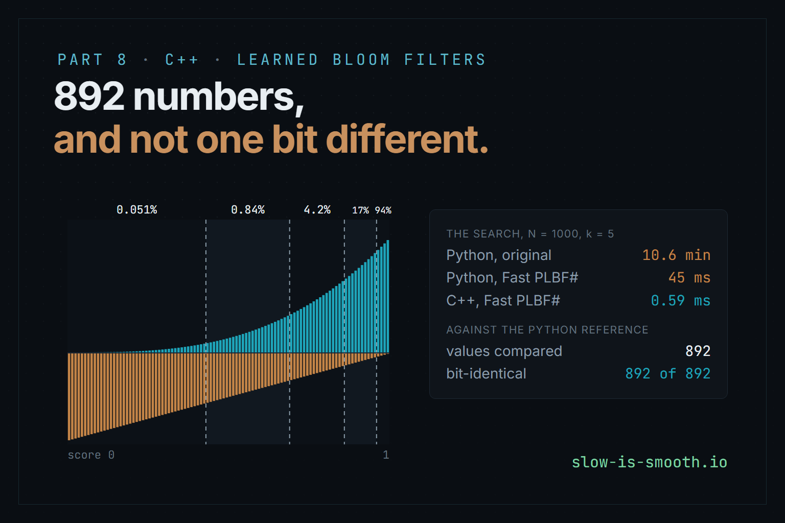
A paper in The VLDB Journal makes a learned Bloom filter’s threshold search up to 75 times faster, and that 75 is not the speed of the search. Timed on its own, the paper’s Python search gets 14,000 times faster, from ten and a half minutes to 45 milliseconds. Ported to C++, the same search takes 0.59 milliseconds. The hard part of the port was not speed. It was getting 892 numbers to agree with the Python reference to the last bit.
Part 8 of the Bloom filter saga: a partitioned learned Bloom filter, from a paper’s Python to header-only C++20, and the tests that held the port to the reference.
This is a guided walkthrough of a port. The paper is Atsuki Sato and Yusuke Matsui’s Fast Construction of Partitioned Learned Bloom Filter with Theoretical Guarantees, published online in The VLDB Journal on 16 October 2026, volume 35, issue 6 (preprint: arXiv 2410.13278v2). It ships a Python reference, FastPLBF. The port is learned-bloom-filter, and every number in this post comes from running it or the reference; the files are named as we go.
The saga so far built a fast, cache-friendly Bloom filter in Go and then spent several parts making it correct under concurrency. This part steps back to a different question: what if the filter could ask a model first? Parts 9 and 10 take the same port into AVX2 and onto a GPU.
How to read this. Where you see a Predict box, stop and answer it before reading on; two of the results here are not what most people guess, and I guessed one of them wrong myself. Of the four figures, the first three are interactive; all four draw only numbers the C++ library produced or the recorded runs measured. Boxes marked “safe to skip” hold the derivations; the main text never depends on them.
What you need to know already: what a hash table is. Bloom filters, dynamic programming over partitions, total monotonicity and SMAWK are all explained where they first matter.
1. A filter that asks a model first
A Bloom filter answers one question, “is this key in the set?”, in very little memory. It is an array of bits, all zero to start. To add a key, hash it a few times and set the bits the hashes point at. To look a key up, hash it the same way and check those bits: if any is zero, the key was never added. If all are set, it probably was, because other keys may have set those same bits between them. That “probably” is the filter’s one weakness, the false positive, and the filter’s one promise is the mirror image: it never says no to a key it holds.
How often it says yes wrongly, the false-positive rate , is set by how many bits it spends per key. With the number of hash functions chosen well, a filter at rate needs
bits per key. At that is 9.59 bits a key, whatever the keys are. That last clause is the opening: a Bloom filter treats every key and every non-key as equally likely, because it knows nothing about them.
Often something does know. Suppose the set is a list of malicious URLs, and you already have a classifier that scores any URL between 0 and 1 for how malicious it looks. The keys mostly score high and harmless URLs mostly score low, though not perfectly: some bad URLs look innocent and some innocent ones look bad. A learned Bloom filter (Kraska et al., 2018) puts that classifier in front of the filter: trust the model where it is confident, and keep a small ordinary Bloom filter, the backup filter, for the keys it would miss, so the one promise still holds.
The partitioned learned Bloom filter, or PLBF (Vaidya, Knorr, Mitzenmacher and Kraska, ICLR 2021), goes one step further. It cuts the score range into regions and gives each region its own backup filter with its own false-positive rate. A region where almost everything scoring there is a key can afford a loose filter, or none at all. A region where keys are rare among many non-keys needs a strict one. Choosing where the regions start and what rate each gets is the whole problem, and the subject of the paper.
Here is what a good choice looks like. The figure uses the two score distributions this series benchmarks with: keys whose scores lean towards 1, and non-keys whose scores lean towards 0, with real overlap in the middle. Every layout it shows is the C++ library’s own output for those settings.
Where the regions fall, and what each one costs
The classifier's score, cut into 100 segments. keys above the line, non-keys below, each scaled to its own tallest bar. Every layout here is the C++ library's own output.
Each band is one region; the label above it is the false-positive rate its backup filter is sized for, and "none" means the region accepts everything that scores into it. Bits are the paper's cost model, a classic Bloom filter at each region's rate; the split-block filters the library builds need roughly a fifth more. The classifier's own size is not counted.
At five regions and a 1% target the filter needs 5.71 bits a key against a plain Bloom filter’s 9.59, 40% less before you count the model. The regions come out uneven: the lowest-scoring region spans almost half the score range at a rate of 0.05%, and the top one, narrow and full of keys, runs at 94%, barely a filter at all.
Predict. Going from 5 regions to 10 should help, since each region can be tuned more finely. How much smaller does the filter get at a 1% target: a quarter, a tenth, or less?
Less. From two regions to five the filter shrinks from 6.88 bits a key to 5.71, but from five to ten only to 5.51, under 4% more. Most of what partitioning can buy, the first few cuts buy. Try the target-FPR pills too: the saving in percent falls as the target tightens, from 71% at 10% to 27% at 0.1%. The box below explains why the saving in bits barely moves at all.
2. Choosing the regions is a search
The paper does not search over arbitrary cut points. It first divides the score range into equal segments, 1,000 by default, and histograms the training data into them: for each segment, the fraction of keys and the fraction of non-keys that score there. A region is then a run of consecutive segments, and a layout is a choice of cut points among the segment boundaries.
From the box above, once the regions are fixed their rates and their cost follow in closed form. So the search is over cut points only, and the quantity to maximise is the divergence : the more the regions separate keys from non-keys, the fewer bits. There is one wrinkle, the clamping. The top region often ends up with no filter at all, and a region at rate 1 contributes nothing to the bits, so the search treats the last region differently: it tries every place where the last region could start, segments to , and for each finds the best regions over segments 1 to . Each candidate then gets its optimal rates and its exact cost, and the cheapest wins.
That inner problem, the best regions over a prefix, is where all the time goes.
3. A table filled in row by row
The best way to cut segments 1 to into regions has a simple structure: its last region runs from some segment to , and everything before it must be the best way to cut segments 1 to into regions. If it were not, swapping in the better prefix would improve the whole. That is the recurrence of a dynamic program, a table filled in one row at a time where each entry reuses entries already filled:
where is the key mass of segments through , read in constant time from prefix sums. Filling the table costs rows, times layers, times up to candidates for : .
The original PLBF does this once for every , which is . That is the paper’s first
observation, and it is almost embarrassing once seen: the table for segments 1 to is just
the first rows of the table for all segments. Fill the big table once and read every
off it. The paper calls this Fast PLBF, and it produces exactly the same answer, to the bit;
in the port it is one function, full_scan_dp in
optimize.hpp,
and the original’s cubic rebuild is kept beside it only so the benchmarks measure what the paper did.
The port changes one more thing. The reference fills each cell by looping over inside a loop over the layer , so it computes the same divergence once per layer. Swapping the two inner loops computes each divergence once and offers it to every layer. Each cell still sees its candidates in the same order under the same comparison, so every value and every recorded split comes out identical; it only stops paying for logarithms where one will do.
4. Row maxima, and the staircase
Fast PLBF is quadratic in . The paper’s two faster methods, Fast PLBF++ and Fast PLBF#, come from looking at one layer of the table as a matrix. Fix the layer , and write : row holds every candidate for the cell , one per starting segment . Filling the layer means finding the maximum of every row, and doing that by scanning every entry is exactly the we already have.
But the maxima have a shape. A region that ends later usually wants to start later too: if the best two-way cut of segments 1 to 9 is before segment 5, the best cut of 1 to 10 is unlikely to be before segment 3. When that holds, the column of each row’s maximum never moves left as you go down the rows. It is a staircase, and the figure shows it.
Finding every row's best split, three ways
Row p: the region ends at segment p. Column i: it starts at segment i. Brighter is closer to the row's best; the outlined cell is the true maximum. Dark cells cannot hold a region.
On the ideal shape the outlined cells step rightwards as you go down: a later end never wants an earlier start. Divide and conquer and SMAWK rely on that staircase to skip most of the matrix. The bumpy shape bends it, and both of them hand back a cell that is not the row's best. The counts are the library's own: repeat visits to a cell count each time.
A staircase lets you skip most of the matrix. Divide and conquer finds the maximum of the middle row by scanning it, then knows every row above has its maximum at or left of that column and every row below at or right of it, and recurses on the two halves. That is per layer, and it is what Fast PLBF++ uses. SMAWK (Aggarwal, Klawe, Moran, Shor and Wilber, 1987) goes further, to : it needs a slightly stronger property, total monotonicity, which says that for any two rows and two columns, if the lower row prefers the right column, so does every row below it. Fast PLBF# uses SMAWK.
When does the staircase actually hold? The paper’s answer is its central theorem. Call the score distribution ideal if the key-to-non-key ratio never decreases as the score rises, which is what a classifier worth having should give you: higher scores, relatively more keys. Under an ideal distribution the matrix is totally monotone, and Fast PLBF++ and Fast PLBF# return exactly what Fast PLBF returns. Under a non-ideal one they can miss a row maximum. For Fast PLBF++ the paper bounds how much memory that can cost, from a measure of how far the distribution is from ideal; for Fast PLBF# it gives no bound and measures the cost instead. Switch the figure to the bumpy shape, where a narrow band of non-keys sits in the middle of the score range, and both fast solvers hand back a cell in row 9 that is not the best.
Predict. SMAWK is linear and divide and conquer is . In the 16-row figure, which of the two evaluates fewer cells?
Divide and conquer, by a lot: 81 cells against SMAWK’s 134, on the ideal shape. Linear time is a statement about large , and SMAWK’s constant is bigger; it evaluates many cells twice, once to reduce and once to interpolate. The crossing point is further out than I expected.
Cells evaluated for one layer, as the number of segments grows
Counted by running the library's solvers; both axes logarithmic.
SMAWK's guarantee is linear and divide and conquer's is N log N, but SMAWK's constant is larger: it only evaluates fewer cells once N passes about 500. At the paper's N = 1000 the two are 8% apart, which is why their measured searches take almost the same time.
SMAWK only drops below divide and conquer between 256 and 512 segments. At the paper’s default of 1,000 the two evaluate 10,974 and 10,059 cells per layer, 8% apart, which is why, as the next section shows, their measured searches take nearly the same time. The full scan’s million is the gap that matters.
5. What the paper’s 75× measures
The paper’s headline numbers are speedups of up to 58.7×, 74.5× and 75.7× for Fast PLBF, Fast PLBF++ and Fast PLBF# over the original, on real datasets (malicious URLs, malware features, DNA k-mers and network-intrusion flows) at and , rising to 235×, 865× and 871× at . Read the caption of its Figure 7 before quoting them: “the construction time includes model training, parameter optimization (i.e., thresholds and FPRs ), and inserting keys into the backup Bloom filters.” It is an end-to-end ratio, and the fixed costs in it, training the classifier and inserting the keys, do not shrink when the search does. The text says the search part directly: the original “takes more than 3 minutes to find the optimal and ”, and the proposed methods do it within 2 seconds on three of the datasets.
So what does the search alone do? I timed the reference’s own Python searches, nothing else, at the
scale of the paper’s URL dataset: 223,088 keys, 428,118 non-keys, , , with
time_reference.py.
All four found the same layout.
$ python -I tools/time_reference.py FastPLBF
time_reference: Python 3.13.9, Intel64 Family 6 Model 183 Stepping 1, GenuineIntel
223088 keys, 428118 non-keys, N = 1000, k = 5, target FPR 0.01; search only, one run each
  search fast_sharp         44.651 ms   backup    1282085 bits   boundary [0, 446, 708, 875, 969, 1000]
  search fast_pp            53.748 ms   backup    1282085 bits   boundary [0, 446, 708, 875, 969, 1000]
  search fast             1155.267 ms   backup    1282085 bits   boundary [0, 446, 708, 875, 969, 1000]
  search plbf           636823.176 ms   backup    1282085 bits   boundary [0, 446, 708, 875, 969, 1000]
Ten and a half minutes for the original, 45 milliseconds for Fast PLBF#: on the search alone the paper’s methods are 551×, 11,848× and 14,262× faster, two orders of magnitude beyond the headline. The headline is not wrong; it answers a different question, how much faster the whole filter gets built, and once the search takes milliseconds, training a classifier takes the rest. On the paper’s DNA dataset, where preprocessing dominates, the same methods cut total construction by only about 25%.
The C++ port runs the same four searches on the same scale of data, in
bench_construct:
The search alone, Python against C++
Milliseconds to find the layout at the paper's URL scale, N = 1000, k = 5. Logarithmic: each gridline is ten times the last.
Measured on one machine on one day. Python is one run each, since the original takes ten minutes; C++ is the median of seven, one run for the original. Within each language the four methods find the same layout; the two languages draw their scores from the same shapes with different random generators, so their layouts differ slightly.
In C++ the original takes 1.5 seconds instead of ten and a half minutes, and Fast PLBF# 0.59 milliseconds instead of 45. On the same algorithm, the change of language alone is worth between 76× (Fast PLBF#) and 416× (the original), the same order as the paper’s end-to-end headline, from a source that has nothing to do with the paper.
Two smaller things in the chart are worth a second look. Fast PLBF++ edges out Fast PLBF# here, 0.54 milliseconds to 0.59: at SMAWK saves 8% of the cell evaluations and spends more than that on its bookkeeping, as the previous section’s counts suggested. And the search is no longer what a build costs. The whole C++ build, histogramming 651,206 scores, searching, sizing the backup filters and inserting 223,088 keys, takes 5.4 milliseconds; the search is about a tenth of it, and the histogram, at 2.6 milliseconds, nearly half.
6. Porting it to the last bit
None of those timings would mean anything if the port computed a different filter. The paper’s guarantees are about this exact algorithm, and the cheapest way to know a port is that algorithm is to compare it with the reference: same inputs, same outputs. The question is how “same” to make it.
I aimed for identical to the last bit, for a practical reason more than a principled one. The search compares sums of logarithms and picks the larger; two layouts within a rounding error of each other are common, and the comparison will pick whichever side the rounding lands on. A port that is merely “close” to the reference can therefore pick a different layout, and then every downstream number differs by far more than an ulp. Agreeing to the bit removes the argument.
Getting there meant copying behaviour that looks incidental:
- Every segment starts with a count of 1. The reference histograms with Laplace smoothing: one imaginary key and one imaginary non-key in every segment. It is load-bearing. It guarantees every segment has some mass of both kinds, so is always finite and no region can end up needing a false-positive rate of exactly zero.
- A score belongs to the segment whose upper threshold it reaches. The reference uses Python’s
bisect_leftover the thresholds , which makes segments open at the bottom and closed at the top, and sends a score of exactly 0 to the first segment. The port stores the same correctly rounded thresholds rather than recomputing them, so a score sitting exactly on a boundary lands on the same side in both. - Ties go left. Every comparison in the reference is strict, so of two equal candidates the first wins. The port’s three solvers do the same.
- The sort is stable. Region rates are assigned in order of key-to-non-key ratio, and Python’s sort
with
reverse=Truekeeps equal ratios in their original order.std::sortwould not;std::stable_sortwith a strict comparison does. - Expressions are evaluated in Python’s order.
normed * (pos / vp) / (neg / vn)is left to right in both, and so is every sum.
The last item has a trap in it. Python rounds after every operation. A C++ compiler, given
prev + pos * std::log(pos / neg) and a target with fused multiply-add, may compute the multiply and
the add as one instruction with one rounding. That is more accurate, and different. I expected that to break
parity with Python, and measured it instead. Rebuilt with -march=native, which lets GCC use FMA, and
-ffp-contract=fast, which lets it fuse wherever it likes, the golden test still matched all 892
values. What broke was a different check. The exact solver computes each transition once and reuses
it across layers, while the approximate ones compute it inline where they need it, so under
contraction the two paths can round the same matrix cell differently, and did. The property “no
approximate DP cell exceeds the exact one”, true by definition in exact arithmetic, failed 2,500
times. Contraction did not make the port disagree with Python on these inputs; it made the port
disagree with itself. The output is in fma_experiment.txt.
The port’s development build passes -ffp-contract=off, and the AVX2 code in Part 9 is compiled with a
per-function target attribute rather than -mavx2, so the optimiser itself never sees an FMA.
The reference became the oracle in the plainest way available: run its own code.
gen_golden.py
imports the reference’s classes, and stubs out pandas, scikit-learn and the bloom_filter package with
empty modules, because those are only used for loading CSVs, splitting data and inserting keys, none of
which the search touches. It then calls each class’s search directly on 116 configurations: the
reference’s own example data at every target its scripts use, plus synthetic ideal and non-ideal data
at 50, 100 and 1,000 segments, 5 and 10 regions, all four methods, and both of the paper’s objectives
(least memory at a target FPR, and least FPR at a memory budget). It writes down every boundary, every
region rate and both costs.
The C++ test reads the same score files, runs the same searches, and demands the boundaries match exactly. It counts the rest:
golden: decisions of the Python reference
  116 cases, 892 values: 892 bit-identical to the reference, worst 0 ulps
That holds under three compilers, g++ 16.1, clang 19.1 targeting x86-64 Windows, and MSVC 19.44. A 32-bit build, whose doubles go through different instructions and a different maths library, lands bit-identical on 804 of the 892 and within 2 ulps on the rest, with every boundary still exact.
Golden cases only cover the inputs someone thought of, so the same test also holds the methods to the paper’s claims on random inputs: the original and Fast PLBF give bit-identical layouts every time; on ideal inputs Fast PLBF++ and Fast PLBF# do too; and on non-ideal inputs no cell of their DP ever exceeds the exact one, and none of their layouts ever needs less memory than Fast PLBF’s. Of 80 random non-ideal cases, 48 got a different layout from the fast methods, and none of those needed less memory.
7. Run it yourself
The figures’ numbers come from the library through a tool, which is one more thing to take on trust. Here instead is the staircase figure’s layer rebuilt from nothing: the same two shapes at 16 segments, the same divergence, and the three solvers written out in under 150 lines, counting every cell they evaluate.
// One layer of the partitioned learned Bloom filter's search, and three ways
// to find its row maxima. N = 16 segments, the post's two score shapes.
//   g++ -std=c++20 -O2 staircase.cpp -o staircase && ./staircase
#include <cmath>
#include <cstdio>
#include <functional>
#include <limits>
#include <vector>

constexpr int N = 16;
const double NEG = -std::numeric_limits<double>::infinity();
using Matrix = std::function<double(int, int)>;  // A(row p, column i), 1-based

// Prefix sums of segment masses: the mass of segments lo..hi is acc[hi] - acc[lo-1].
struct Dist {
    std::vector<double> acc;
    double range(int lo, int hi) const { return acc[hi] - acc[lo - 1]; }
};
template <class Cdf>
Dist masses(Cdf cdf) {
    Dist d{std::vector<double>(N + 1, 0.0)};
    for (int i = 1; i <= N; ++i) {
        const double a = double(i - 1) / N, b = double(i) / N;
        d.acc[i] = d.acc[i - 1] + (cdf(b) - cdf(a));
    }
    return d;
}

// Keys: density 4s^3. Non-keys: density 2(1-s), with `bump` of the mass moved
// into a uniform band [lo, lo + w].
double key_cdf(double s) { return s * s * s * s; }
double non_cdf(double s, double bump, double lo, double w) {
    double band = (s - lo) / w;
    band = band < 0 ? 0 : band > 1 ? 1 : band;
    return (1 - bump) * (1 - (1 - s) * (1 - s)) + bump * band;
}

// The divergence a region over segments i..p adds: pos * ln(pos / neg).
double region(const Dist& g, const Dist& h, double prev, int i, int p) {
    const double pos = g.range(i, p), neg = h.range(i, p);
    if (neg == 0) return NEG;
    return prev + (pos == 0 ? 0.0 : pos * std::log(pos / neg));
}

// Leftmost maximum of row r over columns lo..hi, counting evaluations.
int scan(const Matrix& a, int r, int lo, int hi, long& evals) {
    double best = NEG;
    int arg = lo;
    for (int c = lo; c <= hi; ++c, ++evals) {
        if (const double v = a(r, c); v > best) best = v, arg = c;
    }
    return arg;
}

void full_scan(const Matrix& a, std::vector<int>& out, long& evals) {
    for (int r = 1; r <= N; ++r) out[r] = scan(a, r, 1, N, evals);
}

// Divide and conquer: solve the middle row, then each half within the
// columns a non-decreasing argmax leaves it.
void halve(const Matrix& a, int rlo, int rhi, int clo, int chi, std::vector<int>& out, long& evals) {
    if (rlo > rhi) return;
    const int mid = (rlo + rhi) / 2;
    out[mid] = scan(a, mid, clo, chi, evals);
    halve(a, rlo, mid - 1, clo, out[mid], out, evals);
    halve(a, mid + 1, rhi, out[mid], chi, out, evals);
}

// SMAWK: drop columns that cannot hold a row maximum, solve the odd rows
// recursively, then fill each even row from between its neighbours' answers.
void smawk(const Matrix& a, const std::vector<int>& rows, const std::vector<int>& cols_in,
           std::vector<int>& out, long& evals) {
    if (rows.empty()) return;
    auto f = [&](int r, int c) { ++evals; return a(r, c); };
    std::vector<int> cols;
    for (const int c : cols_in) {
        while (!cols.empty() && f(rows[cols.size() - 1], cols.back()) < f(rows[cols.size() - 1], c)) cols.pop_back();
        if (cols.size() < rows.size()) cols.push_back(c);
    }
    std::vector<int> odd;
    for (size_t i = 1; i < rows.size(); i += 2) odd.push_back(rows[i]);
    smawk(a, odd, cols, out, evals);
    size_t k = 0;
    for (size_t i = 0; i < rows.size(); i += 2) {
        size_t end = cols.size() - 1;
        if (i + 1 < rows.size()) {
            while (cols[end] != out[rows[i + 1]]) --end;  // position of the odd row's answer
        }
        int best = cols[k];
        double best_v = f(rows[i], best);
        for (size_t t = k + 1; t <= end; ++t) {
            if (const double v = f(rows[i], cols[t]); v > best_v) best_v = v, best = cols[t];
        }
        out[rows[i]] = best;
        k = end;
    }
}

void run(const char* name, const Dist& g, const Dist& h) {
    // Layer 1: one region over segments 1..n. Layer 2, the matrix below: the
    // best cut of segments 1..p into two regions, just before segment i.
    std::vector<double> one(N + 1, NEG);
    for (int n = 1; n <= N; ++n) one[n] = region(g, h, 0.0, 1, n);
    const Matrix a = [&](int p, int i) { return i > p ? NEG : region(g, h, one[i - 1], i, p); };

    std::vector<int> exact(N + 1), dc(N + 1), sm(N + 1), rows, cols;
    long e_full = 0, e_dc = 0, e_sm = 0;
    full_scan(a, exact, e_full);
    halve(a, 1, N, 1, N, dc, e_dc);
    for (int i = 1; i <= N; ++i) rows.push_back(i), cols.push_back(i);
    smawk(a, rows, cols, sm, e_sm);

    std::printf("%s: cells evaluated, full scan %ld, divide and conquer %ld, SMAWK %ld\n", name, e_full, e_dc, e_sm);
    for (int p = 1; p <= N; ++p) {
        if (a(p, exact[p]) == NEG) continue;  // no region fits: no maximum to find
        if (dc[p] != exact[p] || sm[p] != exact[p]) {
            std::printf("  row %d: best cut before segment %d, divide and conquer says %d, SMAWK says %d\n", p,
                        exact[p], dc[p], sm[p]);
        }
    }
}

int main() {
    const Dist g = masses(key_cdf);
    run("ideal", g, masses([](double s) { return non_cdf(s, 0.0, 0.69, 0.02); }));
    run("bumpy", g, masses([](double s) { return non_cdf(s, 0.2, 0.4875, 0.0625); }));
}
$ g++ -std=c++20 -O2 staircase.cpp -o staircase && ./staircase
ideal: cells evaluated, full scan 256, divide and conquer 81, SMAWK 134
bumpy: cells evaluated, full scan 256, divide and conquer 81, SMAWK 133
  row 9: best cut before segment 5, divide and conquer says 6, SMAWK says 6
The counts match the figure, 256, 81 and 134 on the ideal shape and 133 for SMAWK on the bumpy one, and so does the miss: row 9’s best two-way cut is before segment 5, and both fast solvers say 6.
8. The takeaway
The paper’s contribution is real and large, and the port is a few hundred lines. But the 75× in its abstract is an end-to-end ratio, and on the search alone the same code is four orders of magnitude faster, fast enough that in C++ the search is no longer the part of a rebuild worth optimising. The interesting cost moved: into the histogram, the key insertion, and the queries, which is where Parts 9 and 10 go.
The port taught a smaller lesson too. “Matches the reference” is a claim with a precision, and the precision that makes it cheap to defend is all of it. Every rule that got the port to 892 out of 892, smoothing, bisect, ties, stable sort, evaluation order, contraction, looked like a detail until a golden case disagreed.
Corrections
While porting, I first logged the reference’s memory-budget mode as having a bug: its _M classes
record the memory of the last candidate they tried, not of the layout they chose. The code does
do that, but every candidate is sized to the same budget, so the two figures differ only in the 16th
significant digit. It is a quirk, not a bug, and the port reports the chosen layout’s memory.
A note on the evidence
Observed. Every timing above was measured on one machine, an Intel i9-13980HX laptop, on 30
October 2026. The Python timings are one run each with Python 3.13.9, because the original method
takes ten minutes; the C++ timings are medians of seven runs, one run for the original. The raw
outputs are committed under
bench/results/2026-10-30/,
with the machine described in its README. The golden comparison and the property checks are
test_optimize, which any of the three compilers above runs in under a second.
The first recording was thrown away. A laptop’s power settings can make it a different machine
a few seconds into a benchmark, and this one did: in the first attempt the CPU throttled within five
seconds of sustained load, and once it took hold the CPU figures came out 2.5 to 10 times slow; the
sections that ran before it were not slow at all. A small probe that prints a compute rate and a memory latency about twice a second showed it,
compute falling from about 1,190 to 160 million operations a second; that trace was read on screen and
not saved. The benchmark outputs are kept in throttled/ as evidence of the failure, never as results;
Part 9 shows what they got wrong. The runs above were recorded after the laptop’s performance mode was set, with
the same probe run before and after them (probe_before.txt, probe_after.txt). They still read 10
to 25% slower than the same benchmarks on the previous day, which is why each comparison in this post
is between numbers from the same run.
Documented, not re-measured. The paper’s speedups, its definition of construction time, the three-minute figure and the 25% on DNA are quoted from arXiv 2410.13278v2. I did not rerun its experiments, which use real datasets and LightGBM models; the data here is synthetic, drawn from the two shapes in the figures.
What differs from the paper’s setup. The paper times its construction in the memory-budget mode; the timings here use the target-FPR mode, which runs the same DP with a different final step. And the filter this port builds is not the paper’s: its backup filters are split-block Bloom filters, which need about a fifth more memory than the classic filters the paper’s cost model assumes. That is Part 9’s subject.
What I would still change. The C++ build is single-threaded, so its histogram and insert steps are slower than they need to be, and the Python timing of the original method is a single run of ten minutes on a laptop.