The Cleaning Robot Puzzle: A Price on Every Move

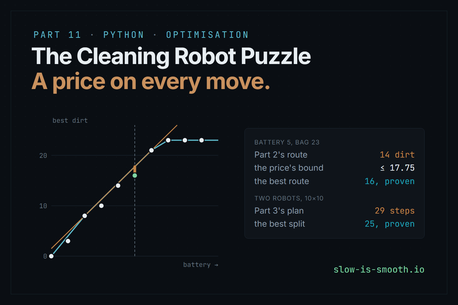
With a battery of five moves, Part 2’s robot collects 14 units of dirt, and the best route collects 16. Charge the robot 3¼ units of dirt for every move it makes, and it can be proved that no route collects more than 17. A drawing shows why no price, however well chosen, can prove 16.

This is Part 11 of the cleaning robot puzzle, and the last of the four parts that restate the robot’s problems the way operations research does. Part 2 gave the robot a battery and solved it with a heuristic, which brute force could check only on tiny rooms. Part 3 gave it a partner and split the work with a fast method, against a lower bound it called weak. Neither said how far from the best its answers were on rooms of any size. This part answers both. The new ideas:

Lagrangian relaxation: put a price on the battery instead of a limit, and every price gives an upper bound;
the inner problem: the best trip at a price, which is Part 10’s pricing problem with dirt as the prize;
subgradient steps, the method that scales to thousands of prices, and two lines, the cutting-plane method that is exact when there is only one;
the duality gap, and the drawing that explains it: a concave hull;
integer programs for walks that may leave fields out: the battery, and the two robots’ split, solved and proven by HiGHS.

File	What it does
`lagrange.py`	the price on a move: the inner problem by labels, subgradient steps, and the exact dual by two lines
`walk_ip.py`	walks that may leave fields out: the battery and the two-robot split as integer programs in HiGHS
`test_lagrange.py`	the checks and the report behind every number below

The labels, the subgradient steps and the two lines are written from scratch; HiGHS, through highspy, solves the integer programs. Every file behind all the parts is listed in the code’s README.

The battery again

Every floor field holds 1 to 5 units of dirt. The robot’s bag holds at most the capacity, and it may make at most battery moves; cleaning a field with C is free. It may finish anywhere, and it should collect as much dirt as it can. This part takes Part 2’s pick-cells rule, under which the robot drives with its brushes up and chooses which fields to clean. As in Part 10, a route is then simply a trip: the fields it cleans, in order, walking the shortest way between them. Its load is the dirt it cleans and its moves are the walk, starting from the dock.

Two budgets make the problem hard. The bag alone is a knapsack, which Part 2 solved exactly with subset sum. The battery turns it into the orienteering problem, which is NP-hard even with no bag at all. Part 2’s heuristic walks towards whatever dirt is most useful per step and decides what to clean at the end. On 800 tiny rooms it matched brute force on 774. On Part 2’s running example with a bag of 23 it misses exactly once:

# # # # # # #
# * 3 4 # 5 #
# 1 5 2 1 5 #
# 4 # 3 2 5 #
# # # # # # #

Battery	3	4	5	6	7
Part 2’s heuristic	10	14	14	21	23
Best route	10	14	16	21	23

With five moves the heuristic takes the 4 next to the start and has nothing useful left to do; the best route, >v>>>, runs along the middle row and collects 3 + 5 + 2 + 1 + 5. On a room this small, brute force can tell. On a room of a hundred fields nothing could, until now. The only upper bound was Part 2’s answer without a battery, which ignores the battery altogether.

A price on every move

Here is the trick. Instead of forbidding the robot to make more than battery moves, charge it: every move costs $\lambda$ units of dirt, and every move it leaves unused earns $\lambda$ back. Then forget the battery. For every price $\lambda \ge 0$ ,

L(\lambda) \;=\; \lambda \cdot \text{battery} \;+\; \max_{\text{trips } t} \big(\text{load}_t - \lambda \cdot \text{moves}_t\big),

where the maximum runs over every trip that fits in the bag, however long. That is an upper bound on every route within the battery. The proof is one line: a route $t$ with $\text{moves}_t \le \text{battery}$ has

\text{load}_t \;\le\; \text{load}_t + \lambda\,(\text{battery} - \text{moves}_t) \;\le\; L(\lambda),

because the bracket is never negative, and $t$ is one of the trips the maximum looks at. This is weak duality, the same inequality that made Part 8’s dual prices a certificate, and $\lambda$ is a Lagrange multiplier: the constraint has been moved into the objective with a price on it.

The price has a meaning: it is how much dirt a move must earn to be worth making. At $\lambda = 0$ moves are free, the battery is forgotten, and the bound is Part 2’s answer without a battery: 23, the whole bag. A huge price makes every move a loss, the best trip is to stay on the dock, and the bound is $\lambda \cdot \text{battery}$ , also huge. In between, the bound dips. With a battery of 5 it is lowest at $\lambda = 3\tfrac14$ . There two trips tie for best: 2 moves that collect 8, and 6 moves that collect 21. Each is worth $8 - 2 \cdot 3\tfrac14 = 21 - 6 \cdot 3\tfrac14 = 1\tfrac12$ , so

L(3\tfrac14) = 3\tfrac14 \cdot 5 + 1\tfrac12 = 17\tfrac34 .

No route with five moves collects more than 17, since dirt comes in whole units. The best collects 16.

Finding the lowest $L$ , over every price, is called the Lagrangian dual. Two questions follow: how to compute $L$ at one price, and how to find the best price.

The inner problem

Computing $L(\lambda)$ means finding the trip that maximises $\text{load} - \lambda \cdot \text{moves}$ with no battery: the inner problem. Walking from field $a$ to field $j$ and cleaning it adds $\text{dirt}_j - \lambda\, d(a, j)$ . That is Part 10’s pricing problem: there each field had a dual price and each move cost one, here each field’s prize is its dirt and each move costs $\lambda$ . The bag is still the resource, and no field may be cleaned twice. lagrange.best_trip uses the same labels: (last field, load, fields remembered, value so far), extended one field at a time. A label is dropped when another at the same field has no more load, no less value and remembers no field it doesn’t:

new = (j, load + inst.dirt[j], (memory & ng[j]) | 1 << j, value + inst.dirt[j] - lam * d[last][j],
       moves + d[last][j], trip + (j,))
bucket = buckets[j]
if any(o[1] <= new[1] and o[3] >= new[3] - EPS and o[2] & new[2] == o[2] for o in bucket):
    continue

On the running example the labels remember every field, so the trips are real and the inner problem is solved exactly. On bigger rooms they remember only the 8 nearest, Part 10’s ng-routes, and a trip may then come back to a field it cleaned long ago and count its dirt twice. That can only raise $L$ , so the bound stays a bound.

Relaxing the battery did not make the inner problem easy, only easier: it is still NP-hard, and it has one resource fewer than the problem it bounds. That is the usual bargain. Lagrangian relaxation pays off when what is left has structure an algorithm can use, and here that structure is Part 10’s labels. Low prices need care. Near $\lambda = 0$ every way of walking a load is worth almost the same, so the labels hardly dominate each other, and the first version took minutes for a single price. Two changes fixed it. The search starts with Part 2’s answer without a battery as the best trip so far, which at low prices is nearly the best there is. And a label is dropped when even filling the rest of its bag for free couldn’t beat that:

if new[3] + Q - new[1] <= best[0] + EPS:
    continue                                # can't beat the best even with a free full bag

Points and lines

Every trip is a point: its moves across, its load up. At a price $\lambda$ , the trip contributes the line

\text{load}_t + \lambda\,(\text{battery} - \text{moves}_t),

and $L(\lambda)$ is the highest of all those lines. A maximum of straight lines is convex and piecewise linear: it bends only where the best trip changes. Its slope at $\lambda$ is $\text{battery} - \text{moves}$ of the trip that is best there. If that trip is longer than the battery the slope is negative, and raising the price lowers the bound. If it is shorter the slope is positive, and lowering the price lowers the bound. The best price is where the slope changes sign.

Turn the same picture around. For every battery $b$ , let $f(b)$ be the most dirt any route with $b$ moves can collect: a staircase that rises and then flattens out at the bag. The price draws a line of slope $\lambda$ that lies above every point of the staircase, and $L(\lambda)$ is that line’s height at the battery. The lowest such line, over every slope, touches the staircase’s concave hull: the smallest bent-down curve that lies above every point. So the Lagrangian dual is not some new number. It is exactly the concave hull of the best answers, at the battery:

\min_{\lambda \ge 0} L(\lambda) \;=\; \hat f(\text{battery}).

On the running example the staircase is 0, 3, 8, 10, 14, 16, 21, 23, … and the hull’s corners are at 0, 2, 6 and 7 moves. With a battery of 5 the hull runs straight from (2, 8) to (6, 21) and passes 17¾. The best route, 16, sits below it, and nothing a single price can do will reach down there.

Deep divesafe to skip on a first read

Why the dual is the hull

One direction. Pick any $\lambda \ge 0$ . The line $y = L(\lambda) - \lambda\,\text{battery} + \lambda b$ lies above every point $(b, f(b))$ , because $f(b) - \lambda b \le \max_t(\text{load}_t - \lambda\,\text{moves}_t)$ for every $b$ . A line above every point lies above the hull too, since the hull is the lowest concave curve above the points and a line is concave. So $L(\lambda) \ge \hat f(\text{battery})$ for every price.

The other. The hull is made of straight pieces between corners of the staircase. At the battery, take the piece that covers it and the price equal to its slope. That line passes through two corners and lies above every other point, so the highest line at that price is this one, and $L$ equals the hull there.

What it says. The dual sees the staircase only through its hull. Where the battery falls on a corner, as 6 does, the price proves the best route. Between corners it can’t, and the difference between the hull and the staircase is the duality gap. It comes from whole numbers: moves can’t be split, so the robot can’t make “half of the 2-move trip and half of the 6-move trip”, which is exactly the point on the hull the dual sees.

Tested. On 60 tiny rooms, at every battery, the exact dual equalled the hull of Part 2’s brute-force answers. On 13 of the 244 batteries tried, the hull was a whole unit or more above the best route, so no price could prove it.

Two ways to find the best price

Subgradient steps

The slope of $L$ at the current price says which way to go, even where $L$ has a corner and no true derivative; there any slope between the two sides will do, and such a slope is called a subgradient. lagrange.subgradient starts at what a move earned on Part 2’s route and steps against the slope:

\lambda \;\leftarrow\; \max\!\Big(0,\; \lambda - \theta\,\frac{L(\lambda) - \text{low}}{g^2}\, g\Big), \qquad g = \text{battery} - \text{moves},

where $\text{low}$ is the best route found so far. Polyak’s step size, the fraction, is how far the price would have to move for $L$ to reach $\text{low}$ if it were the straight line through this step. $\theta$ starts at 1 and halves after three steps that don’t improve the bound. Every inner trip is cut where the battery runs out, and that gives a real route, which may raise $\text{low}$ :

value, trip, moves, load = best_trip(inst, lam)
bound = lam * battery + value
cut = within(inst, trip, battery)
if inst.load(cut) > low:
    low_trip, low = cut, inst.load(cut)
...
g = battery - moves
if best < low + 1 - 1e-6 or g == 0:
    return best, low_trip, k
lam = max(0.0, lam - theta * (bound - low) / (g * g) * g)

It stops when the bound proves the best route found, since loads are whole numbers, or when the slope is 0, because then no price does better. Otherwise it stops after a fixed number of steps. On the running example with a battery of 4, it proves 14 in 5 steps. With a battery of 5 it zigzags round 3¼, and after 30 steps, or 60, its best is 17.766: close to 17¾ but never on it. It also has no way of knowing how close it is. That is the price of a method that needs only one slope at a time: it is what scales to a thousand prices, where nothing better is known, and it is slow to finish.

Two lines

With a single price there is something much better. Every trip found is a line below $L$ . Keep the best line that rises, from a trip within the battery, and the best that falls, from one over it. The minimum lies where they cross, so solve the inner problem there. If no trip lies above both lines at the crossing, the crossing is the minimum. Otherwise the new trip’s line replaces the one on its side. lagrange.dual starts with the empty trip, whose line rises, and Part 2’s answer without a battery, whose line falls:

for k in range(1, 200):
    (m1, l1), (m2, l2) = rise, fall
    lam = Fraction(l2 - l1, m2 - m1) if exact else (l2 - l1) / (m2 - m1)    # where the two lines cross
    level = lam * (battery - m1) + l1
    value, trip, moves, load = best_trip(inst, lam)
    if lam * battery + value <= level + (0 if exact else 1e-7):
        return level, lam, k + 1
    if moves <= battery:
        rise = (moves, load)
    else:
        fall = (moves, load)

In exact fractions it finds 71/4 at the price 13/4 in four steps, and stops because it knows it has arrived. This is Kelley’s cutting-plane method for a convex function, and it is also Part 10’s column generation seen from the other side. Each trip is a column; the two lines are a master program with two columns; the inner problem is pricing. The Lagrangian dual and the linear program over all trips have the same value. That is why the history box below belongs to both parts.

What is a move worth?

Part 2's room with a bag of 23. Every route is a point: its moves and its dirt. A price per move turns every point into a line, and the highest line at the battery is a bound no route can beat.

Battery

Method

the trip that is best at this price

bound against price

best dirt against battery

Step

Price per move

Bound

Best route so far

trip within the battery trip over the battery concave hull the price's line the best route

History

Everett, Held and Karp, and the subgradient

Hugh Everett, better known for the many-worlds interpretation of quantum mechanics, showed in 1963 that a price on a scarce resource turns a constrained allocation problem into an unconstrained one, and that whatever the priced problem chooses is optimal for the budget it happens to use (Everett, 1963). Michael Held and Richard Karp made the idea famous on the travelling salesman problem. They put a price on every city, relaxed “every city has two neighbours”, and were left with a minimum spanning tree on all but one city plus that city’s two cheapest edges, which is easy (Held and Karp, 1970; 1971). With Philip Wolfe and Harlan Crowder, Held then showed that simple steps against a subgradient find good prices fast (Held, Wolfe and Crowder, 1974); the step size used here is Boris Polyak’s, with the best route found standing in for the optimum he assumed was known (Polyak, 1969). Arthur Geoffrion named the method Lagrangean relaxation and proved how its bound compares with a linear program’s (Geoffrion, 1974), and Marshall Fisher’s survey made it a standard tool (Fisher, 1981). The cutting-plane method for the dual is James Kelley’s (Kelley, 1960). The robot’s inner problem, a path under a resource with the other resource priced, is the classic way to solve the constrained shortest path problem (Handler and Zang, 1980; Beasley and Christofides, 1989).

Closing the gap

The duality gap is a fact about the hull, so no cleverer price can close it. Something has to look inside the hull, at whole-number routes, and Parts 9 and 10 have shown two ways to do that: branch, or list everything that could still win. This part writes the battery as an integer program and lets HiGHS do both.

The model is Part 9’s walk, with one change: the walk no longer has to reach every field. walk_ip.py gives it a variable $y_v$ per field, 1 if the walk reaches it, and keeps Part 9’s rules for what it reaches. $x_e$ counts the walks along each pair of neighbours, $z_v$ marks where the walk ends, and parity holds at every field:

\begin{aligned} & x_e \le 2\,y_v \ \text{ for both ends } v \text{ of } e, \qquad z_v \le y_v, \qquad x(\delta(v)) + z_v \ge 2\,y_v \ \ (v \ne s), \\ & \text{the start sends one unit of flow to every reached field, along walked pairs only}, \\ & \textstyle\sum_e x_e \;\ge\; \sum_v y_v - 1 \qquad \text{(at most one new field per move)}. \end{aligned}

The flow is Part 9’s compact way of saying “connected”: a walk in pieces can’t carry it. For the battery, add $c_v \le y_v$ for the fields it cleans, and

\text{maximise } \sum_v \text{dirt}_v\, c_v \quad\text{such that}\quad \sum_v \text{dirt}_v\, c_v \le \text{capacity}, \qquad \sum_e x_e \le \text{battery}.

HiGHS starts from Part 2’s route, so it has something to beat, and proves the best on every battery of the running example in a fraction of a second. The program’s linear relaxation is another upper bound, and it is instructive to put it beside the price’s:

Battery	1	3	4	5	6
Best route	3	10	14	16	21
The price’s bound	4	11¼	14½	17¾	21
The program’s linear relaxation	3	11	14	17	23

Neither is always better. Geoffrion’s theorem says a price is at least as strong as the linear relaxation of the same model, because the inner problem keeps the trips whole while the linear program lets everything be fractional. But these are two different models. The price relaxes only the battery and keeps every route whole; the walk program keeps the battery and lets the walk be fractional. With a battery of 6 the price proves the best route and the linear program is 2 short of doing so; with 1, 3 and 5 it is the other way round.

On rooms of real size the comparison tips one way. Random rooms with 30% furniture and dirt from 1 to 5, with a bag big enough that the battery is what binds; the price remembers 8 fields and takes 30 subgradient steps:

Rooms	Part 2’s heuristic	The program’s linear relaxation	The price’s bound	Best route	Proven	Proven by the price alone	Part 2’s route is the best
6 of 8×8, bag 40, battery 10	24.3	27.5	26.0	25.8	6 of 6	5 of 6	2 of 6
6 of 10×10, bag 60, battery 15	50.3	58.7	56.3	54.8	6 of 6	2 of 6	2 of 6
4 of 12×12, bag 80, battery 20	54.8	66.2	63.5	58.8	4 of 4	1 of 4	1 of 4

The numbers are means over the rooms. In every group the price’s bound sits well below the linear relaxation’s: on bigger rooms most of the slack is in letting the walk be fractional, and that is exactly what the price never does. On half the rooms the price alone proves the best route, in 2 to 14 seconds on average; HiGHS proves every one, in 2 to 28 seconds on average. Part 2’s heuristic, which matched brute force on 97% of tiny rooms, finds the best route on only 5 of these 16. On average it is 1.5 to 4.5 units short, about 6 to 8%. The answer Part 2 couldn’t give is that its battery heuristic is good, but not as good as tiny rooms made it look.

Two robots

The question again

Part 3’s second robot shares the room. Robot A starts on * and robot B on @. Every step both run their next command at the same time, the floor is clean once one of them has been on every field, and the time is the longer of the two command strings. They must not collide. Part 3 split the work three ways, by regions, by cutting one shared walk, or by giving everything to one robot, and kept the fastest. Then it planned one robot around the other in space and time. Its exact search over (A’s field, B’s field, cleaned fields) stopped at about 14 fields. On 12×12 rooms its plans were 1.19 times its lower bound, and the bound, at most two new fields per step, was known to be weak. Was the plan slow, the bound weak, or both?

Two walks and a clock

walk_ip.two_robots gives each robot its own copy of the walk above, starting on its own field, adds a whole number $T$ for the time, and asks for the smallest:

\text{minimise } T \quad\text{such that}\quad y^A_v + y^B_v \ge 1 \ \text{ for every field } v, \qquad T \ge \sum_e x^A_e, \qquad T \ge \sum_e x^B_e .

Two more rows help the linear relaxation, since a robot can’t reach a field before it has walked there: $T \ge d(s_k, v)\, y^k_v$ for both robots and every field. Part 3’s plan goes in as the first answer, and its time $U$ does a second job: a robot can’t reach a field more than $U$ moves from its start in a plan that beats it, so those $y$ are fixed at 0 from the start.

Minimising the larger of two numbers is a notoriously weak model. The linear relaxation splits every field half and half and balances the two walks perfectly, so it rarely says more than “half the fields each”, which is Part 3’s own bound. Everything else comes from HiGHS’s branching and its cuts. The program also lets the robots share a field, which is what Part 3’s first step did too, so its answer is a lower bound on any plan that keeps them apart. Collisions are then handled exactly as in Part 3, by walk_ip.no_collisions, which runs Part 3’s step 2 on any plan. When the plan it returns takes no longer than the best sharing plan, it is the best plan without collisions as well.

The best split

Random rooms with 0, 15 or 30% furniture, as in Part 3, with five minutes for each program:

Rooms	Fields (mean)	Part 3’s bound	The program’s linear relaxation	Part 3’s plan	Best split found	Proven best	Time (mean)
6 of 8×8	25	11.8	12.5	13.3	13.3	6 of 6	2 s
6 of 10×10	56	27.2	27.5	29.7	28.8	6 of 6	30 s
4 of 12×12	87	42.5	43.0	47.2	45.0	2 of 4	200 s

The times are steps until the room is clean. The two 12×12 rooms that weren’t proven end 3 and 1 steps above HiGHS’s bounds. The plans are the sharing ones, and keeping the robots apart cost nothing: run through Part 3’s step 2, every best split above finished in the same time, so on the proven rooms it is the best plan without collisions too.

So Part 3’s question, slow plan or weak bound, has the answer “both, and it depends on size”. On 8×8 rooms Part 3’s plans are already the best there is, every one, and only the bound was short, by 1.5 steps on average. On 10×10 the plans are 0.9 steps off on average, about 3%, and the bound 1.6 short. On 12×12 the plans are at least 2.2 steps off, about 5%, and the bound at least 1.5 short. The linear relaxation adds less than a step to Part 3’s bound, as a model that minimises the larger of two numbers would predict; HiGHS’s branching does the rest, and on 12×12 it runs out of time.

Two robots, split two ways

A furnished 10×10 room. Robot A starts on the teal field, robot B on the copper one; each tints the fields it cleans. Both plans keep the robots from colliding.

Time

Fields left

Done at

robot A and what it cleans robot B and what it cleans

Deep divesafe to skip on a first read

A price on every field

Decomposition. The two robots are tied together by one family of rows: every field must be reached by one of them. Put a price $\pi_v \ge 0$ on each of those rows instead, and fix the time $T$ . The problem falls apart into one problem per robot: which fields are worth reaching within $T$ moves, if field $v$ pays $\pi_v$ ? That is Part 2’s battery problem, with prices for dirt, $T$ for the battery and no bag. If, at some prices, the fields both robots can collect within $T$ moves pay less than the sum of all the prices, then no plan finishes within $T$ . This is Lagrangian decomposition, and it is the reason the method is used at all: a problem with a few coupling rows becomes many small problems and one price vector, which subgradient steps can tune with thousands of prices.

Why this part doesn’t compute it. Each robot’s problem has no bag, and without one nothing stops the labels’ ng-routes from going round and round collecting the same distant prices again. They would need the battery $T$ as a resource after all. The bound the prices give would also be no better than column generation over pairs of routes, Part 10’s method with one route per robot. By the same theorem as the two lines, a Lagrangian dual and the linear program over the inner problem’s solutions are the same number seen from two sides.

Testing Part 11

test_lagrange.py produces every number above:

Check	How
The inner problem	150 tiny rooms with random prices, against every trip there is: remembering every field the labels find the best one; remembering one, never a worse one
The dual	60 tiny rooms, every battery: the exact dual equals the concave hull of Part 2’s brute-force answers
Subgradient steps	60 tiny rooms: never below the dual, every route they report replayed by Part 2’s simulator; 56 reached the dual, the rest ended at most 0.80 above it
The battery program	80 tiny rooms: proven best, equal to Part 2’s brute force, every route replayed; the linear relaxation never below the best
The two-robot program	60 tiny rooms: proven best, equal to Part 3’s exact search and its independent referee; the plan made collision-free replayed with collisions forbidden, never faster than Part 3’s exact answer
The figures	`docs/check_or_figures.py` reruns the subgradient steps and the two lines, checks every bound the page draws against the labels, and replays both two-robot plans, in Chromium

What Part 11 teaches

A price turns a limit into a trade-off. Charge for what is scarce, drop the limit, and every price gives a bound: weak duality in one line.
What is left must be easier, not easy. The inner problem is still NP-hard. It has one resource fewer, and Part 10’s labels already solve it.
Subgradients scale; cutting planes finish. One slope at a time works with a thousand prices and never knows it has arrived; with one price, two lines get there exactly.
The gap is a picture. The dual sees the best answers only through their concave hull, so where the battery falls between two corners, no price can prove the best route.
Compare bounds by what they relax. The price keeps routes whole and the linear program keeps the battery; each wins where the other gives most away.
Decompose along the coupling rows. Two robots tied by “every field cleaned once” become two battery problems as soon as each field has a price.

That closes the four parts that set out to measure Parts 2 and 3 against the best. Part 8 bounded the fewest commands from below, and Part 9 proved the shortest routes. Part 10 proved the best plans for emptying the bag. This part bounded the battery from above, proved its best routes, and proved the best split between two robots. Each time the earlier fast answer turned out to be good, never more than about an eighth from the best, and each time its bound, where it had one, was further off than the answer was. Most of the work of a proof turned out to be the work of a bound.

The battery again

A price on every move

The inner problem

Points and lines

Two ways to find the best price

Subgradient steps

Two lines

Closing the gap

Two robots

The question again

Two walks and a clock

The best split

Testing Part 11

What Part 11 teaches

Subscribe

More