The Cleaning Robot Puzzle: A Room That Wraps Around
 The Cleaning Robot Puzzle: A Room That Wraps Around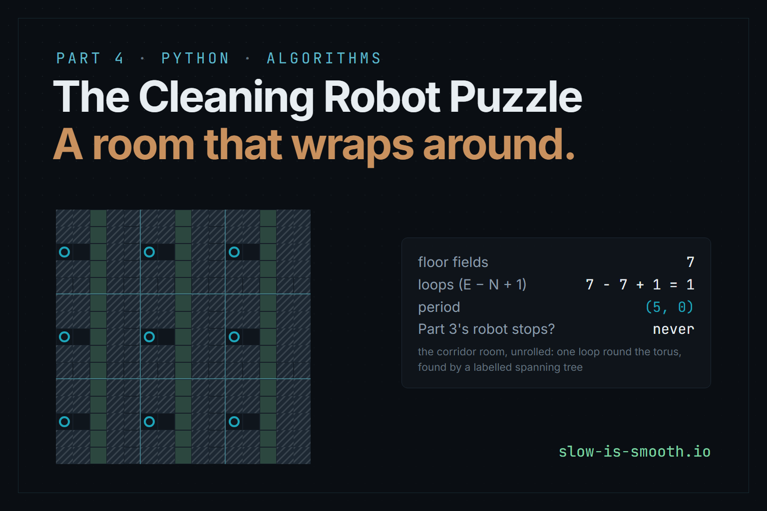
Contents
Glue the cleaning robot’s room into a doughnut, so that walking off the right edge brings it back on the left, and the blind robot from Part 3 never stops cleaning.
This is Part 4 of the cleaning robot puzzle, and the first of four parts in which the floor stops being flat. Part 1 cleaned a room with a depth-first walk, Part 2 added dirt, a bag and a battery, and Part 3 asked for the fewest commands, took the map away, added a dock and a second robot. Every one of those rooms was a flat grid with a wall round it.
The next four parts keep the square fields and glue them together differently:
| Part | The floor | What the flat grid gave for free, and loses |
|---|---|---|
| 4 (this one) | a room that wraps round both ways, a torus | positions worked out by counting moves; the checkerboard |
| 5 | a strip with a twist, a Möbius strip | a compass: ^ no longer means the same thing everywhere |
| 6 | the walls of a box | corners: three left turns can bring the robot home |
| 7 | a floor with five squares at every corner | room: the number of fields within reach grows exponentially |
Each part also teaches algorithms and data structures that Parts 1 to 3 never needed, because the new floor is what makes them necessary. This one needs four:
- a spanning tree whose edges carry labels, with the loops that the edges outside the tree close (a cycle basis);
- the Hermite normal form, a canonical way to write down a lattice of whole-number vectors;
- a two-colouring that returns an odd loop when it fails, a certificate anyone can check;
- the doubling trick, the answer to searching when you don’t know how far to look.
The code is Python, as before, and every file is served next to the post:
| File | What it does |
|---|---|
surface.py | square fields glued edge to edge, the robot’s moves and a simulator; shared by Parts 4 to 7 |
torus.py | the room that wraps around, Part 1’s walk on it, random rooms and a robot object for the blind tests |
periods.py | the labelled spanning tree, the room’s periods and the Hermite normal form |
blind_torus.py | a blind robot that finishes, with a dock it can recognise |
two_colour.py | a checkerboard colouring, or an odd loop that proves there isn’t one |
route_exact.py | fewest commands on any surface, with the checkerboard pruning optional |
test_surface.py, test_torus.py | simulators, referees and the report behind every number below |
Every file behind all the parts is listed in the code’s README.
The room that wraps around
The room is still a list of strings, one character per field, with # for furniture, . for floor and * for the robot’s start. There is no wall round the edge any more. Walking off the right edge brings the robot back on the left edge of the same row, and walking off the bottom brings it back on the top of the same column. The commands are still ^ v < >, and there is still a budget of 50,000 of them.
This is the geometry of the arcade game Asteroids, where anything that leaves one side of the screen reappears on the opposite side, top and bottom as well as left and right. Pac-Man’s tunnel only wraps left to right. Glue only one pair of edges and you get a tube, a cylinder. Glue both and you get the surface of a ring doughnut, a torus:
The arrows on the edges are the way topologists draw it: edges with the same arrows are glued together, arrow to arrow. Roll the square into a tube so the single arrows meet, then bend the tube round so its two ends meet, and the double arrows meet too.
Nothing is wrong with the torus as a floor. It is flat in the sense that matters to the robot: every corner has four squares round it, and a small patch of it looks exactly like a patch of the old grid. What changes is the whole, not the parts. A walk that keeps going > comes back to where it started. So does a walk that keeps going ^, and, sooner or later, one that goes >^>^>^… for ever. The flat room had loops too, round furniture, but none that went round the room.
The best way to see a torus is to unroll it. Lay copies of the room side by side in every direction, like tiles on a bathroom wall, and the robot’s moves become steps on an endless plane. Every field of the room appears once in every copy. Drive the robot below and watch both pictures at once:
One torus, an endless plane of copies
Drive the robot with the buttons or the arrow keys. On the left it is on the torus; on the right, at the position it would count, on the plane of copies.
The room, edges glued
Unrolled: nine copies round the robot's copy
On the plane the robot’s position is two whole numbers, how far it has gone down and across since it started, counted in fields. On the torus those numbers only matter modulo the room’s height and width. Five rows high means ^ five times is back where you started, and the plane shows it as a copy of the start one room further up.
Part 1’s walk still works
Given the map, cleaning the torus is no harder than cleaning a flat room. Part 1’s walk steps into every unvisited neighbour and steps back when it is stuck. It needs to know each field’s neighbours and nothing else, and on a torus the neighbours wrap:
DIRS = [(-1, 0, '^', 'v'), (1, 0, 'v', '^'), (0, -1, '<', '>'), (0, 1, '>', '<')]   # Part 1's table


def solution(room):
    R, C = len(room), len(room[0])
    start = next((r, c) for r in range(R) for c in range(C) if room[r][c] == '*')
    seen, moves = {start}, []

    def dfs(r, c):
        for dr, dc, go, back in DIRS:
            nr, nc = (r + dr) % R, (c + dc) % C      # the only change from Part 1
            if room[nr][nc] != '#' and (nr, nc) not in seen:
                seen.add((nr, nc))
                moves.append(go)
                dfs(nr, nc)
                moves.append(back)

    dfs(*start)
    return ''.join(moves)
The % R and % C are the whole difference. Part 1’s proof goes through unchanged too. The walk visits every field it can reach, uses each edge of its tree twice, and so costs exactly 2(N − 1) commands for N floor fields. In torus.py the same walk runs on surface.py, the square-field model that Parts 5 to 7 need, and on 500 random rooms up to 15×15 the simulator confirmed every field cleaned in exactly 2(N − 1) commands.
That is worth saying out loud, because it tells us where to look. An algorithm that only asks “who are my neighbours?” can’t tell a torus from a flat room with some extra doors. The trouble starts where an algorithm leans on something more: on positions it works out itself, or on a fact about flat grids that it never checks. Part 3 had one of each.
The blind robot never stops
Part 3’s blind robot has no map. It has one sense: robot.move(d) either moves one field and returns True, or bumps into something, stays put and returns False. To build a map, it calls its starting field (0, 0) and names every other field by the position it works out from counting its own moves. It stops when every field it knows has been probed on all four sides.
On a flat room that is exactly right. Each field has one position, and the robot’s map is the room.
On a torus, one field has infinitely many positions: (0, 0), (5, 0), (−5, 0), (0, 7), (5, 7) and so on for a 5×7 room, one for each copy on the unrolled plane. The robot can’t know that the field at (5, 0) is the field at (0, 0). Every field looks the same to it: floor or not floor, and nothing else. So it treats (5, 0) as a new field, probes round it, finds more new fields, and keeps going. The room it believes in is not the torus but the endless plane of copies, and it is trying to clean all of it.
Here is the smallest room I know where that happens. A corridor runs round the torus from top to bottom, and the dock sits at the end of a short side passage:
Part 3’s robot walks right into the corridor, turns up it, and never comes back. It tries ^ first, and there is always more floor above, so every call is another step up. After 20,000 move calls its map holds 19,996 fields, nearly all of them one corridor climbing up the page. The room has seven.
It doesn’t always happen. Here is a room whose floor is a ring round a pillar, walled in on the torus:
Part 3’s robot cleans its eight fields and stops, exactly as on a flat floor. The loop round the pillar is a loop, but it doesn’t go round the torus: walked on the unrolled plane, it comes back to the same copy of the start. The corridor’s loop comes back to a different copy, five rows up.
That is the whole story, and it can be said precisely. Walk any loop on the torus, starting and ending on the same field, and follow the same moves on the unrolled plane. You end up in some copy of your starting field, shifted by some whole number of room heights down and room widths across. Call that shift the loop’s period. The ring round the pillar has period (0, 0); the corridor has period (5, 0), or (−5, 0) walked the other way. Part 3’s robot stops exactly when every loop in the floor has period (0, 0). One loop with a non-zero period is enough to make its map endless.
Which loops go round the room?
With a map, the question “does any loop go round the torus?” has a clean answer, and computing it is this part’s first new algorithm.
A spanning tree with labels
Label every step with how far it moves the robot on the unrolled plane: (−1, 0) for ^, (1, 0) for v, (0, −1) for < and (0, 1) for >. Now run a breadth-first search from the start, as in Part 2’s box on the subject, and give each field a position: the start gets (0, 0), and a field first reached by a step from field f gets f’s position plus that step’s label. The edges the search used form a spanning tree, and each field’s position is where its tree path from the start ends on the plane.
The steps the tree did not use are where the loops are. A non-tree step from field f to field g closes exactly one loop: g’s tree path back to where it meets f’s, then f’s tree path down to f, then the step. Going round that loop on the plane ends at
which is the loop’s period. In periods.py:
def spanning_tree(room):
    R, C = len(room), len(room[0])
    start, floor = parse(room)
    position = {start: (0, 0)}
    parent = {start: None}
    queue = deque([start])
    loops = []
    while queue:
        cell = queue.popleft()
        y, x = position[cell]
        for dy, dx in STEP.values():
            n = ((cell[0] + dy) % R, (cell[1] + dx) % C)
            if n not in floor:
                continue
            if n not in position:
                position[n] = (y + dy, x + dx)
                parent[n] = cell
                queue.append(n)
            elif parent[n] != cell and parent[cell] != n and cell < n:
                ny, nx = position[n]
                loops.append((cell, n, (y + dy - ny, x + dx - nx)))
    return position, loops
The cell < n test counts each non-tree step once, from its smaller end. On the corridor room the search finds one non-tree step, from the top of the corridor to the bottom, with period (−5, 0). On the pillar room it finds one too, with period (0, 0).
Click any dashed step below to see the loop it closes and that loop’s period:
Every step outside the tree closes one loop
The breadth-first tree is solid. Click a dashed step to see the loop it closes and how far round the torus that loop goes.
Why the tree’s loops are enough
A room has many more loops than non-tree steps: go round the pillar twice, or round the corridor and then the pillar. But every loop is built from the tree’s loops. Walk any loop and, each time it uses a non-tree step, swap that step for the tree’s loop through it. The tree parts cancel out, because a tree has no loops of its own, and what is left is the original loop written as a sum of fundamental cycles, one per non-tree step. Periods add up along the way, so every loop’s period is a sum of the fundamental cycles’ periods, each counted a whole number of times, some of them negatively.
A graph with N fields and E edges has a spanning tree with N − 1 of them, so there are E − N + 1 fundamental cycles. That number is the graph’s cyclomatic number, and the fundamental cycles are a cycle basis: in the language of linear algebra, a basis of the space of all loops. It costs one breadth-first search to find.
The lattice of periods, and a canonical name for it
The periods of all loops form a lattice: every sum and difference of periods is the period of some loop, so the set is closed under adding and subtracting. Rooms differ in how big their lattice is:
- Rank 0: only (0, 0). No loop goes round the room. The floor unrolls into separate copies of itself, one per tile, and Part 3’s robot finishes.
- Rank 1: all multiples of one vector, like (5, 0) for the corridor. The floor unrolls into infinite strips, and the robot’s map runs off along one of them.
- Rank 2: all whole-number combinations of two independent vectors. The floor unrolls into one endless connected sheet.
One lattice can be spanned by many different lists of vectors. (5, 0) and (0, 7) span the same lattice as (5, 7) and (10, 7), or as (5, 0), (0, 7), (5, 7) and (10, −7) together. To compare two lattices, or to tell whether a new period is really new, we need one canonical way to write each lattice down. For vectors of whole numbers that is the Hermite normal form: every lattice in the plane has exactly one basis of the shape
or a smaller one of the same kind when the rank is lower. Finding it is Euclid’s algorithm run on whole vectors instead of numbers:
def hermite(vectors):
    top, ds = None, []
    for v in vectors:
        v = list(v)
        if v[0] == 0:
            ds.append(v[1])
            continue
        if top is None:
            top = v
            continue
        while v[0] != 0:                    # Euclid on the first entries, carrying the second
            q = top[0] // v[0]
            top, v = v, [top[0] - q * v[0], top[1] - q * v[1]]
        ds.append(v[1])
    d = 0
    for y in ds:
        d = gcd(d, y)
    basis = []
    if top is not None:
        if top[0] < 0:
            top = [-top[0], -top[1]]
        if d:
            top[1] %= d
        basis.append(tuple(top))
    if d:
        basis.append((0, d))
    return tuple(basis)
Euclid’s step replaces the larger of two numbers by its remainder modulo the smaller, and here each step subtracts a whole vector, so the second entries come along. Every subtraction stays inside the lattice and can be undone, so the lattice never changes. When the first entries are exhausted, everything left has first entry 0, and the gcd of the second entries is d. Finally b is reduced modulo d, which is the step that makes the answer unique.
The same basis also gives each position a canonical representative, reducing the first entry modulo a and then the second modulo d:
def reduce(p, basis):
    y, x = p
    for a, b in basis:
        if a:
            k = y // a
            y, x = y - k * a, x - k * b
        else:
            x %= b
    return y, x
Two positions differ by a period exactly when they reduce to the same pair. That is what lets a robot name a field once it knows the periods, in the next section.
The prediction
So the map predicts the blind robot: compute the lattice of periods, and Part 3’s robot stops exactly when its rank is 0. On 600 random rooms from 3×3 to 12×12, with up to 60% furniture, the rank was 0 on 127, 1 on 134 and 2 on 339. Run with a limit of 20,000 move calls, Part 3’s robot stopped on exactly the 127 rooms of rank 0, with the right number of fields every time, and ran into the limit on all the others.
No robot can know it has finished
Is Part 3’s robot just badly designed? Could a cleverer robot, with the same single sense, clean a torus and stop?
No. Take any room whose floor has a loop that goes once round the torus from top to bottom, like the corridor. Now build a second room twice as tall, the first room stacked on a copy of itself. Its floor is still one connected piece, because that loop now runs through both copies. But to a robot with a bump sensor the two rooms are identical: every field has the same neighbours, floor or not, in both, and nothing marks which copy it is in. So any robot, however it decides, makes exactly the same moves and gets exactly the same answers in both rooms, move for move, for as long as it runs.
Now suppose some robot always cleans every field and then stops. On the first room it stops after some number of moves T. Stack k copies instead of two, with k chosen so that the tall room has more than T + 1 fields. The robot receives the same readings there, so it stops after the same T moves, having visited at most T + 1 fields. Some field is left dirty. So no such robot exists.
The test builds that doubled room for 262 random rooms with a loop round the torus, runs Part 3’s robot in both, and compares the logs: identical, move for move, for all 20,000 calls. The argument is the covering space again. The robot’s senses can’t tell a room from its covers, so it can’t tell which cover it is in, and the covers have no largest member.
A dock the robot can recognise
The way out is to give the robot a sense that can tell the copies apart. Real robots have one: they come back to a dock, and they know when they are on it. So robot.on_dock() now says whether the robot is standing on its dock, the field it started on, and there is only one dock.
Now a loop round the torus announces itself. When the robot stands on the dock at a counted position other than (0, 0), it has just walked a loop, and the counted position is that loop’s period. The robot adds it to its lattice with hermite. From then on it names every field by its position reduced modulo the lattice, and the part of its map it has already built folds up: positions that differ by a period merge into one field.
That idea, recognising a place you have been before and correcting your map accordingly, is what real mapping robots call loop closure.
Exploring frontier first
Part 3’s robot explored depth first, walking back along its trail when it was stuck. This robot explores the way many real robots do: frontier first. The frontier is every known floor field that still has a neighbour nobody has probed. The robot walks, over floor it knows, to the nearest such field and probes it. Brian Yamauchi introduced frontier-based exploration for mobile robots in 1997 (Yamauchi, 1997). When there is no frontier left, the whole folded map has been explored and it is done.
On its own, frontier first has the same flaw as Part 3’s robot. In the corridor room, once the robot is in the corridor, the nearest unprobed neighbour is always the next field up. The robot probes it, steps into it, and repeats, climbing an endless-looking corridor for ever and never going back to look down the side passages where the copies of the dock are. Run with no limit on 100 random rooms with a loop round the torus, it was still going on 36 of them after ten times as many move calls as the version below needed in the same room.
The doubling trick
The fix is to limit how far from the dock the robot may go, and to raise the limit when it gets in the way:
def solution(robot, group=None, growth=2, radius=1):
    group = group if group is not None else Lattice()
    known = {group.canon((0, 0)): True}     # name of a field -> True floor, False furniture
    pos = (0, 0)
    stats = {'periods': 0, 'doublings': 0}
    while True:
        near = dock_distances(known, group)
        target = nearest_frontier(pos, known, group, near, radius)
        if target is None:
            if not any(near[name] >= radius for name in frontier(known, group, near)):
                stats['radius'] = radius
                return sum(known.values()), stats
            radius *= growth                # the limit stopped it: look further
            stats['doublings'] += 1
            continue
        path, d = target
        for step in path:                   # over known floor to the frontier field
            assert robot.move(step)
            pos = shift(pos, step)
        n = shift(pos, d)
        known[group.canon(n)] = robot.move(d)
        if not known[group.canon(n)]:
            continue                        # bumped into furniture
        pos = n
        reading = robot.on_dock()
        assert reading or group.canon(pos) != group.canon((0, 0)), 'map says dock, robot says not'
        if reading and group.learn(pos, reading):
            stats['periods'] += 1
            known = fold(known, group)
dock_distancesis a breadth-first search over known floor from the dock, giving each known field its distance.nearest_frontieris a breadth-first search from the robot, over known floor, for the nearest field within distanceradius − 1of the dock that still has an unprobed neighbour. It returns the path there and the direction to probe.groupis the lattice of periods, whosecanonreduces a counted position to the field’s name, and whoselearnadds a period when the dock turns up somewhere new.foldrenames every field in the map by the new lattice, merging the ones that turn out to be the same. The assertion inside it checks that merged fields agree about being floor or furniture, which they must if the map is right.
When the limit is the only thing stopping the robot, the radius doubles and exploration goes on. When nothing is left to probe at any distance, the folded map is the whole room.
Why is this guaranteed to finish? While the lattice is missing a period, the map extends infinitely in some direction, and there is a copy of the dock at some finite distance D on it. Every frontier field within the radius gets probed, so once the radius passes D the robot reaches that copy and learns something new. The lattice can only grow a few times. Every period the robot learns belongs to the floor’s own lattice, and each time the learned lattice grows, either its rank goes up or its cell shrinks to half its area or less, while the floor’s lattice sets a floor under that area. Once the learned lattice is complete, the folded map is exactly the room, finite, and exploring it ends. When nothing is left to probe, every field reachable in the folded map has been visited, and any missing period would have shown up as a copy of the dock among them.
Watching it think
The figure runs both robots on the corridor room: Part 3’s on the left and the new one on the right. Each is drawn twice, on the real torus below and on its own map above, where every field is named by its counted position. Part 3’s map grows up the corridor without end. The new robot’s map grows too, until it finds the dock at (10, 0), two laps down the corridor. It learns the period (10, 0) and folds its map, and later it finds the dock at (5, 0) and folds again, to the seven real fields:
Two blind robots, one corridor
Above each room, the robot's own map: every field named by the position it counted. The room has seven floor fields.
Part 3's robot
its map
the real room
With a dock it recognises
its map
the real room
Why two laps before one? The robot reached the side passage one lap down after 46 calls, but the dock’s copy there was one step beyond the radius at the time, so it couldn’t probe it. By the time the radius doubled, the robot was further down the corridor, and the nearest unprobed field was the passage two laps down. Folding by (10, 0) and then by (5, 0) is correct, just slower than finding (5, 0) straight away. In all it used 63 moves and 29 bumps to clean the seven fields.
Results
On 400 random rooms from 3×3 to 14×14, with up to 55% furniture, the dock robot cleaned every field and stopped every time, and the lattice it learned was exactly the room’s lattice of periods, as periods.py computes it from the map. It also cleaned all the fields of each room’s doubled version from the proof above, the one with a single dock, where Part 3’s robot can’t tell the two rooms apart: this robot notices that the dock isn’t where the smaller room would have put it.
It pays for its safety in walking. Moves per field, counted as moves divided by N − 1 so that Part 1’s walk scores 2:
| Rooms | How many | Moves per field, average | Worst | Periods learned, average |
|---|---|---|---|---|
| no loop round the torus (rank 0) | 76 | 2.83 | 4.00 | 0 |
| loops round one way (rank 1) | 89 | 4.12 | 11.80 | 1.11 |
| loops round both ways (rank 2) | 235 | 4.41 | 9.90 | 2.06 |
On the rank-0 rooms, where Part 3’s robot works, Part 3’s best variant (trimmed, with shortcuts) walked 1.84 moves per field against this robot’s 2.83. Both bumped every wall touching the floor exactly once. So on rooms that don’t wrap, not knowing whether the room wraps costs about half as much walking again, and that is the price of the radius: the robot keeps coming back towards the dock before it knows it needn’t.
Why double, and not triple? A separate sample of 400 random rooms, with the radius growing by different factors (moves per field, averaged by rank, and the worst single room):
| Radius grows | Rank 0 | Rank 1 | Rank 2 | Worst room |
|---|---|---|---|---|
| ×2 | 2.71 | 4.34 | 4.30 | 12.30 |
| ×3 | 2.50 | 4.18 | 4.03 | 12.62 |
| ×4 | 2.27 | 3.70 | 3.66 | 19.03 |
| ×8 | 2.21 | 3.98 | 4.53 | 17.94 |
Larger factors spend less on rooms that don’t wrap, because the robot turns back less often. Factor 4 is best on average for rooms that do. Doubling has the best worst case, though tripling comes close, and factors 4 and 8 let one unlucky room cost half as much again. As with the cow, the choice is between the average and the worst, and the measurements show both. They also show why the sample has to be large: an earlier run on 150 rooms, before the report had a fixed seed of its own, put tripling’s worst case ahead of doubling’s.
The checkerboard breaks
The other place Part 3 leaned on flatness is less visible. Its fewest-commands solver proved routes optimal with a lower bound, and part of that bound was a checkerboard: colour the floor like a chessboard, and every command steps onto the other colour. With S fields sharing the start’s colour and O fields of the other colour, a route needs at least 2S − 2 and at least 2O − 1 commands. The exact solver used the same count to cut its search short.
The colouring was (row + column) mod 2. On a torus whose sides are both even that still works. But walk across a 3-wide room with >>> and you are back where you started after three steps: from light to dark to light to dark, on a field you already know is light. An odd number of steps round the torus breaks the colouring.
Here is the smallest case, an empty 3×3 torus with the robot in the middle of the left edge:
The start is on a light field, with four light fields and five dark ones, so Part 3’s bound says the route needs at least 2 · 5 − 1 = 9 commands. But ^^>^^>^^ cleans all nine fields in 8. The bound is wrong, and so is any “proof” of optimality built on it.
The exact solver is hurt too, because it throws away partial routes that the bound says can’t win:
Seven fields. The best route is >>^<<^, 6 commands. Part 3’s search, run with wrapped neighbours and trusting (row + column) mod 2, pruned that route away and returned ^^v<v<^, 7 commands, as the best.
Colour the floor, or prove you can’t
The fix is to stop assuming the colouring and build it instead. Breadth-first search from the start already gives every field its distance; colour each field by whether its distance is even or odd. Neighbours then have distances that differ by at most one. If two neighbours have the same colour, their distances are equal, and their two tree paths back to where they meet, plus the step between them, form a loop of odd length:
def two_colour(surface, start):
    depth = {start: 0}
    parent = {start: None}
    queue = deque([start])
    while queue:
        f = queue.popleft()
        for g in neighbours(surface, f):
            if g not in depth:
                depth[g] = depth[f] + 1
                parent[g] = f
                queue.append(g)
            elif depth[g] % 2 == depth[f] % 2:
                return 'odd loop', odd_loop(parent, depth, f, g)
    return 'colours', {f: d % 2 for f, d in depth.items()}


def odd_loop(parent, depth, a, b):
    left, right = [a], [b]
    while a != b:
        if depth[a] >= depth[b]:
            a = parent[a]
            left.append(a)
        else:
            b = parent[b]
            right.append(b)
    return left + right[-2::-1]
An odd loop can’t be coloured with two colours, since the colours would have to alternate all the way round and arrive back wrong. So when the colouring fails, the loop is a certificate: anyone can check it, by confirming that consecutive fields are neighbours and that its length is odd, without trusting the search that found it. The test does exactly that for every odd loop it gets. On the 3×3 torus, the certificate is the three fields of the left column: down, down, and down again is home.
Try other sizes below. The colouring breaks along the seam whenever a side is odd, and the figure shows the odd loop the search finds:
Does the checkerboard close up?
An empty torus coloured like a chessboard. Make a side odd and the colours clash across the glued edge; the search then hands back an odd loop.
The periods predict the colouring
The periods already know whether the floor is bipartite. A step changes a field’s position on the plane by one in one coordinate, so it changes the sum of the two coordinates by one, and a loop’s length has the same parity as its period’s two entries added: a loop with period (5, 0) has odd length, one with period (5, 7) even length. A loop with period (0, 0) has even length, because it is also a loop on the unrolled plane, which is a flat grid. So the floor has an odd loop exactly when some period has an odd sum, and the test checks that prediction against the two-colouring: on 600 random rooms, 248 could be coloured and 352 had an odd loop, every certificate checked, and the periods predicted which on every one.
That is the first sign of an idea that returns in Parts 5 and 6. A step’s label (−1, 0) says how far it moves on the plane. Keep only the sum of its entries modulo 2, and the label says whether it changes colour. The spanning tree is the same, the labels live in a smaller group, and the same loop arithmetic answers a different question.
Fewest commands, again
With the colouring built by the search, the exact solver in route_exact.py prunes with the checkerboard when there is one and without it when there isn’t. On 816 small rooms (up to 13 fields, tori 3 to 5 rows high and 3 to 6 wide), it agreed with a brute-force search that prunes nothing, every time, and the simulator accepted every route. Trusting (row + column) mod 2 instead, as Part 3 did, overstated the lower bound on 263 of those rooms and pruned the best route away on 77.
Testing Part 4
As in Parts 2 and 3, every claim above comes from test_torus.py, which runs in a couple of minutes:
| Check | How |
|---|---|
| Part 1’s walk on a torus | 500 random rooms up to 15×15, replayed on the simulator: every field, exactly 2(N − 1) commands |
| The Hermite normal form | 3,000 random lists of vectors: every input reduces to zero, the cell area matches the gcd of the 2 × 2 determinants, order and redundant inputs don’t matter |
| The prediction | 600 random rooms: Part 3’s robot stops within 20,000 calls exactly when the rank is 0 |
| Covers | 262 rooms and their doubles: identical move logs for 20,000 calls |
| The dock robot | 400 rooms and their doubles: every field, and the learned lattice equals the map’s |
| No radius | 100 rooms with a loop round the torus: frontier first without a limit is still going on 36 after ten times the calls the doubling robot needed |
| Two colours | 600 rooms: a colouring or a checked odd loop, as the periods predict |
| Fewest commands | 816 small rooms: pruned search equals brute force; Part 3’s colouring fails on 263 and 77 |
test_surface.py checks the shared model underneath. On 505 flat rooms, Part 1’s walk run through surface.py produces exactly Part 1’s commands. Every gluing is symmetric, every torus, cylinder, strip and box has the right Euler characteristic, and the walk cleans every field on 1,506 surfaces of every kind.
What Part 4 teaches
- Find out what an algorithm really uses. Part 1’s walk asks only for neighbours, so it doesn’t care that the room is a torus. Part 3’s blind robot uses positions it works out itself, and the fewest-commands solver uses a colouring it never checks. Those are the parts that broke.
- Label the edges, and the spanning tree does the rest. One breadth-first search with displacement labels finds every loop’s period, predicts whether the blind robot stops, and predicts the checkerboard.
- Canonical forms make comparisons trivial. The Hermite normal form turns “is this new period really new?” into comparing two tuples.
- Some things can’t be known, and a proof says so. No robot with only a bump sensor can clean a torus and stop, because it can’t tell the room from its covers. The fix is a new sense, not a cleverer program.
- A failure can carry its own evidence. The two-colouring either colours the floor or hands over an odd loop that anyone can check.
- When you don’t know how far to look, double. The radius costs a constant factor and guarantees an answer. How big that factor should be is a trade-off between the average and the worst case, and it can be measured.
Part 5 glues the room’s edges with a twist, and the robot loses its compass.