The Cleaning Robot Puzzle: Five Squares at Every Corner
 The Cleaning Robot Puzzle: Five Squares at Every Corner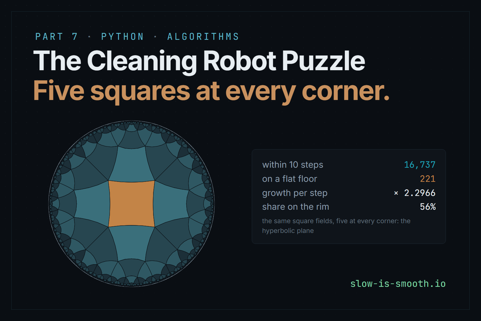
Contents
Put five squares round every corner of the cleaning robot’s floor instead of four, and within ten steps of the dock there are 16,737 fields instead of 221.
This is Part 7 of the cleaning robot puzzle, and the last of four in which the floor stops being flat. In Part 6, three squares met at the corners of a box, each corner was 90° short, and three left turns brought the robot home. This part goes the other way. Five squares meet at every corner, each corner has 90° too many, and the floor, which can no longer lie flat, turns out to have room for far more fields than any flat floor.
Nothing about a single field changes: it is still a square with four neighbours, and the robot still drives from one to the next. What changes is how many fields there are within reach, and that one number reaches into everything Parts 1 to 3 took for granted. The new algorithms:
- building the floor exactly, ring by ring, with nothing but whole numbers, because the usual way, with coordinates, quietly goes wrong;
- a transfer matrix, raised to a power by repeated squaring, that counts the fields in ring 1,000 without building any of them;
- Berlekamp–Massey, which finds the rule behind a sequence of numbers from its first few terms;
- searching from both ends, which on a flat floor saves about half the work and on this floor saves more the further you search.
| File | What it does |
|---|---|
hyperbolic.py | the floor built exactly, ring by ring; the same floor from floating-point coordinates, for comparison |
growth.py | the transfer matrix, fast powers, and the growth rate |
berlekamp_massey.py | the shortest linear recurrence behind a sequence |
bidirectional.py | breadth-first search from one end and from both |
surface.py | the square-field model, the robot and the simulator from Parts 4 to 6 |
test_hyperbolic.py | the checks and the report behind every number below |
Every file behind all the parts is listed in the code’s README.
Five squares at every corner
Try it with paper squares. Put four round a point and they lie flat. Put five and the fifth doesn’t fit: the corner has 450° of paper for the 360° a flat sheet has room for, so it buckles. Keep going, five at every corner, and the sheet ruffles more and more at its edges, like a lettuce leaf or a coral. That ruffled sheet is a patch of the hyperbolic plane.
In 1997 Daina Taimiņa, at Cornell, found that crochet makes sturdy physical models of it: increase the number of stitches in each row by a fixed ratio and the fabric ruffles in exactly this way (Cornell Chronicle; her book is Crocheting Adventures with Hyperbolic Planes). Since 2005 Margaret and Christine Wertheim’s Crochet Coral Reef has crocheted whole reefs of the stuff, because corals, kelps and sea slugs grow ruffles much like it.
Regular tilings are written {p, q}: regular p-sided tiles, q of them at every corner. Squares four at a corner are {4, 4}, the flat floor. {4, 3} is a cube, three at a corner, curved like a sphere. {4, 5} is this floor. For tiles with p, q ≥ 3 the rule is simple: (p − 2)(q − 2) less than 4 gives a sphere-like shape, equal to 4 the flat plane, more than 4 the hyperbolic plane (Mosseri, Vogeler and Vidal, 2022). For {4, 5} it is 2 × 3 = 6.
It can’t be drawn flat without distortion, but it can be drawn faithfully in the Poincaré disc, where the whole infinite floor fits inside a circle. Every field there is the same size and every corner the same shape, but fields near the rim are drawn smaller and smaller, and straight lines are drawn as circular arcs that meet the rim at right angles. Click a field to put it at the centre:
An infinite floor inside a circle
Every field here is the same size; the disc draws those near its rim smaller. Five squares meet at every corner.
Click any field near the start to move it to the middle.
The same robot
Locally, nothing has changed. The robot is on a square field with four neighbours, and it drives with its own directions, carrying its frame over each edge as in Parts 5 and 6. Part 1’s walk, run on surface.py, cleans a round room of this floor with furniture in it exactly as it cleaned everything else: on 40 random round rooms, every reachable field in exactly 2(N − 1) commands.
The corners are where it shows. Drive one field, turn left, and repeat. On a flat floor that closes after four stretches, round a box’s corner after three. Here every corner has five squares, so it closes after five, from every field and every starting direction (180 loops checked), and the robot comes home a quarter turn round, the other way from on the box. Every corner is 90° short on a box and 90° over here: curvature of the opposite sign.
Drive it below. On the open floor, Play drives one field, turns left and repeats, and after five stretches the robot is home with its ^ pointing where its > did. In the round room, Play runs Part 1’s walk round seven pieces of furniture: 38 fields, 74 commands. Follow the robot keeps it in the middle of the disc, so the floor slides past underneath it, and every field it reaches looks just like the one it left.
Driving where five squares meet at every corner
The same robot, with the same four neighbours on every field, carrying its own directions over every edge. Only the corners are different.
^
its > side
its ^ at the start
where it has been
the corner five left turns go round
furnitureSo this floor has no compass either, for the same reason as the box: loops turn the robot. But the box was finite and mostly flat. This floor is infinite and curved at every corner, and that is what makes it grow.
Curvature, counted
Part 6 checked every box against Descartes: the corners’ defects, 360° minus 90° for each square there, add up to 360° times the Euler characteristic. Here every corner inside the floor has five squares, a defect of −90°, so a round room’s inside corners add up to a large negative total. A round room is a disc, with Euler characteristic 1, so its rim has to make up the difference, 360° more than the inside takes away:
| Round room of radius r | Fields | Corners inside | Their defects | Corners on the rim | Rim’s share | Total |
|---|---|---|---|---|---|---|
| 1 | 5 | 0 | 0° | 12 | 360° | 360° |
| 2 | 17 | 4 | −360° | 28 | 720° | 360° |
| 3 | 45 | 12 | −1,080° | 68 | 1,440° | 360° |
| 5 | 257 | 80 | −7,200° | 356 | 7,560° | 360° |
| 8 | 3,169 | 1,008 | −90,720° | 4,324 | 91,080° | 360° |
On a flat floor the rim of a round room turns through 360°, once round, and that is all. Here the rim of a room of radius 8 turns through 91,080°, the rim of a disc ruffled like a lettuce leaf, and it has 4,324 corners on it, more than the room has fields. That is the same fact as “more than half the room is its outer ring”, seen from the curvature’s side.
A step is not a unit of distance
In the smooth hyperbolic plane, a disc of radius ρ has area 2π(cosh ρ − 1), which grows like πe^ρ. Neighbouring fields’ centres are 2a ≈ 1.0613 apart, with cosh a = cos 36° / sin 45°, so one might expect the fields within r steps to grow by e^{1.0613} ≈ 2.890 per step. They grow by 2.297.
The difference is that a step is not a straight line. A field r steps away is at most 1.0613 r away as the crow flies, so the fields within r steps all lie inside a disc of that radius, and their number can grow at most like 2.890^r. But most of them are much closer than that, because a path of steps zigzags from field to field, and the disc of steps is thinner than the disc of distance. Counting in steps is the robot’s view; counting in distance is the geometer’s. The first is what the robot’s commands cost, so it is the one that matters here.
How many fields are within r steps?
On a flat floor, the fields exactly r steps from the start form a diamond with 4r fields, so there are 2r² + 2r + 1 within r steps: 221 within 10. Here:
| r | Flat floor | Five squares at a corner | Share in the outermost ring |
|---|---|---|---|
| 1 | 5 | 5 | 80% |
| 2 | 13 | 17 | 71% |
| 3 | 25 | 45 | 62% |
| 5 | 61 | 257 | 58% |
| 8 | 145 | 3,169 | 56.5% |
| 10 | 221 | 16,737 | 56.5% |
| 11 | 265 | 38,445 | 56.5% |
| 12 | 313 | 88,301 | 56.5% |
| 15 | 481 | 1,069,697 | 56.5% |
| 20 | 841 | 68,346,797 | 56.5% |
The rings hold 1, 4, 12, 28, 64, 148, 340, 780, 1792, 4116, 9452, … fields. Each is about 2.2966 times the one before. That is exponential growth, and the flat floor’s is only linear in r. The sequence is in the On-Line Encyclopedia of Integer Sequences as A377322, “number of cells that are a distance of n away in an order-5 hyperbolic square tiling”, with the same growth.
Fields within r steps of the start
Flat floor against five squares at every corner. The dashed line is the most Part 1's 50,000-command walk can clean.
The numbers
| r | flat | five at a corner |
|---|
The rest of this post is about how to get those numbers exactly, and what they do to the problems of Parts 1 to 3.
Building the floor exactly
The usual way to build a hyperbolic tiling is with coordinates. Put the start field’s centre at the origin of the hyperboloid model, where points are triples (x, y, z) with x² + y² − z² = −1, and step to a neighbour with a fixed 3 × 3 matrix: a rotation by a multiple of 90° and a “boost” by the distance between neighbouring centres. Multiply matrices out along each path, and recognise a field you have reached before by its centre, rounded to a few decimal places. hyperbolic.py has that version as float_layers, and to ring 10 it agrees with everything below.
But rounding is the weak point. The coordinates of a field r steps away grow exponentially with r, and the rounding error of a double-precision number is about 2⁻⁵² times its size, so the error in a far field’s centre grows exponentially too. Walk n steps straight out and n steps straight back in floating point, and see how far from the origin “home” ends up:
| Steps out and back | Largest error at “home” (20 walks) |
|---|---|
| 5 | 7 × 10⁻¹³ |
| 10 | 9.9 × 10⁻⁸ |
| 15 | 0.00092 |
| 20 | 0.5 |
| 30 | 0.5 |
By 20 steps nothing of the calculation is left: the answer is rounded to halves. Recognising fields by rounded centres fails in a subtler way first. Rounded to six decimal places, the float construction first miscounts at ring 15, with 603,948 fields instead of 603,932: sixteen fields computed along two different paths landed on centres that rounded differently, and were counted twice. Rounding to nine places, more precise, fails earlier, at ring 10: 9,456 instead of 9,452. Finer rounding splits one field’s slightly different computed centres into two names sooner. No number of digits is safe for long, because the errors grow exponentially too.
The disc figure near the top of this post builds its fields the same way, and its first version made a mistake of its own at ring 2, not ring 15: it counted 14 fields there instead of 12. It named each centre by printing it to six decimal places, and JavaScript prints a coordinate of −10⁻¹⁷ as -0.000000 and one of +10⁻¹⁷ as 0.000000. One field, two names. Python’s round returns −0.0, which is equal to 0.0 and hashes the same, so the Python version never showed the problem. The figure checker caught it by comparing the page’s counts with the exact ones. The driving figure does it the other way round: it builds its fields as the next section does, and uses coordinates only to draw them.
Ring by ring, with whole numbers
The exact construction never computes a coordinate. It builds the patch of all fields within n steps of the start, and keeps one thing about its boundary: the ring of corners round it, in order, and for each corner how many of its five squares are already there. The next ring of fields is exactly the fields across the patch’s boundary edges, since a field n + 1 steps away shares an edge with one n steps away, and those corners say how the new fields fit together:
- A corner that is missing only one square gets one new field, which covers both boundary edges on either side of it: a notch fills in.
- A corner missing two gets two new fields, one across each boundary edge, which meet along a new edge from the corner and complete it.
- A corner missing three or more also gets two new fields, but they don’t meet: the corner stays on the new boundary, with two more squares than before.
Every new field has one or two fields of the previous ring beside it, its parents: one when it sits across a single boundary edge, two when it fills a notch. The new corners are numbered as they are made, so nothing is ever made twice, and nothing needs to be recognised.
for n in range(1, depth + 1):
    gap = {v: q - deg[v] for v in boundary}
    # Start the ring at a corner that is missing at least two squares.
    i0 = next(i for i, v in enumerate(boundary) if gap[v] >= 2)
    ring = boundary[i0:] + boundary[:i0]
    m = len(ring)
    # Runs: stretches of boundary edges that one new field covers, split at corners missing
    # two or more squares.
    cut = [i for i in range(m) if gap[ring[i]] >= 2]
    runs = []
    for a, b in zip(cut, cut[1:] + [cut[0] + m]):
        runs.append([ring[i % m] for i in range(a, b + 1)])
    ...
Each run of boundary edges between two corners missing two or more squares becomes one new field. A run of one edge gives a field with two new corners; a run of two edges, a notch, gives a field with one. The rest of rings creates the new corners, shares one between the two fields that meet at a corner missing exactly two squares, lists each new field’s corners in order round it, and reads off the new boundary.
The checks are strict, because a construction like this is easy to get subtly wrong:
- Built out to ring 9 (7,285 fields), every one of the 2,320 corners inside the patch has exactly five squares, every edge belongs to at most two fields, and the patch has Euler characteristic 1, a disc.
- Glued into a
surface.pysurface by shared corners, a breadth-first search from field 0 gives every field its ring number as its distance, and each field’s parents are exactly its neighbours one ring closer. - The counts agree with the floating-point construction ring for ring to ring 14.
To ring 12 (88,301 fields) it takes a third of a second.
Counting without building
The construction only needs one number per boundary corner, how many squares it has so far. So count the boundary corners touched by one, two, three and four squares: call those counts a, b, c and d. The three rules above say what happens to each kind:
- A corner touched by one or two squares is missing three or more. It gets two new fields, stays on the boundary touched by three or four, and sends out two new edges whose far ends are new corners touched by one square each.
- A corner touched by three is missing two. Its two new fields meet along one new edge, whose far end is a new corner touched by two.
- A corner touched by four is a notch. One new field fills it, and the two new edges that its neighbours would have sent out end at the same corner, so two new corners become one.
Put together:
and the next ring has a + b + c fields, one for every corner missing two or more squares. The rule is a 4 × 4 matrix, and counting ring r means multiplying by it r − 1 times, starting from a single square’s four corners, (4, 0, 0, 0). The test checks the rules against the real construction, corner by corner, on the first twelve rings.
RULE = ((2, 2, 0, -1),
        (0, 0, 1, 0),
        (1, 0, 0, 0),
        (0, 1, 0, 0))
START = (4, 0, 0, 0)                # one square: four corners, each touched by one


def mat_pow(m, n):
    """m to the n-th power by repeated squaring: about 2 log2(n) multiplications."""
    result = tuple(tuple(int(i == j) for j in range(4)) for i in range(4))
    while n:
        if n & 1:
            result = mat_mul(result, m)
        m = mat_mul(m, m)
        n >>= 1
    return result


def shell(r):
    """Fields exactly r steps from the start, from the matrix alone."""
    if r == 0:
        return 1
    v = mat_pow(RULE, r - 1)
    a, b, c, _ = (sum(v[i][j] * START[j] for j in range(4)) for i in range(4))
    return a + b + c
Repeated squaring computes RULE¹⁰⁰⁰ with about twenty matrix multiplications instead of a thousand, and Python’s whole numbers never overflow: ring 1,000 has a number of fields 362 digits long. Nothing is built.
The growth rate, exactly
How fast does it grow? A matrix raised to high powers is dominated by its largest eigenvalue, the largest root of its characteristic polynomial. For this matrix that polynomial, computed with exact integers by the Faddeev–LeVerrier method (Urbain Le Verrier devised it in 1840 to study the orbits of the planets; Rehman and Ipsen tell its history), is
Its coefficients read the same backwards, so dividing by x² and writing y = x + 1/x turns it into y² − 2y − 2 = 0, a quadratic, with y = 1 + √3. Solving x + 1/x = 1 + √3 gives the growth rate:
The other roots are 0.4354 and a pair of complex numbers of size exactly 1, which don’t grow at all. So the rings grow like λ^r, and the ratio of ring 60 to ring 59 agrees with λ to twelve digits.
The matrix says more than the growth rate. Its eigenvector for λ gives the mix of corner types the boundary settles into, whatever it started from: 58.6% of the boundary’s corners are touched by one square, 11.1% by two, 25.5% by three and 4.8% are notches, touched by four. By ring 12 the real boundary (70,460, 13,360, 30,680 and 5,816 corners) matches those shares to four digits. A boundary that looks the same at every scale is one reason the growth is so regular: each ring is, in proportion, a copy of the one before, 2.2966 times longer.
That also gives the share of a round room in its outermost ring. The ring is about λ^r and everything inside it about λ^r / (λ − 1), so the outer ring holds a fraction 1 − 1/λ ≈ 56.46% of the room, at every radius past a handful. On a flat floor the outer ring of a room of radius r holds 4r of about 2r² fields, a share that shrinks to nothing. Here, more than half of any round room is its rim.
Finding the rule from the numbers
Suppose you didn’t know the four rules, only the counts: 1, 4, 12, 28, 64, 148, … Is there a rule behind them, and what is it?
Berlekamp–Massey answers that. Given the first terms of a sequence, it finds the shortest linear recurrence sₙ = c₁sₙ₋₁ + c₂sₙ₋₂ + … + c_L sₙ₋L that produces all of them. It reads the terms one at a time, keeping the best recurrence so far. When the next term disagrees with the prediction, it corrects the recurrence using the last recurrence that failed, scaled so that the mistake cancels, and only makes the recurrence longer when it has to:
def berlekamp_massey(seq):
    """Returns [c1, ..., cL], as Fractions, for the shortest recurrence the terms satisfy."""
    s = [Fraction(x) for x in seq]
    c, b = [Fraction(1)], [Fraction(1)]        # connection polynomials, current and last
    L, m, last = 0, 1, Fraction(1)
    for n in range(len(s)):
        d = s[n] + sum(c[i] * s[n - i] for i in range(1, L + 1))   # how wrong c is here
        if d == 0:
            m += 1
            continue
        coef = d / last
        t = list(c)
        c = c + [Fraction(0)] * (len(b) + m - len(c))
        for i, bi in enumerate(b):
            c[i + m] -= coef * bi
        if 2 * L <= n:
            L, b, last, m = n + 1 - L, t, d, 1
        else:
            m += 1
    return [-x for x in c[1:L + 1]]
With exact fractions there is no rounding anywhere, and given 2L terms of a sequence that really follows a recurrence of length L, the answer is that recurrence. Fed the nine ring counts from ring 1 to ring 9, it returns
whose characteristic polynomial is x⁴ − 2x³ − 2x + 1: the same as the matrix’s. The recurrence then predicts rings 10 to 14 exactly. (It needs four starting terms, so it holds from ring 5 on; the start field itself, ring 0, doesn’t follow it, as the OEIS entry also notes.)
The two derivations are independent: one comes from the geometry of corners, the other from nothing but the numbers. Their agreement is the strongest check in this part.
What exponential growth does to Parts 1 to 3
The algorithms of Parts 1 to 3 work on this floor unchanged, since they only ask about neighbours. What changes is how much there is.
Part 1’s budget. The original puzzle allowed 50,000 commands, and Part 1 observed that the budget was enormous: the depth-first walk needs at most 2(N − 1) commands, and a 40 × 40 room has at most 1,444 floor fields. On a flat floor, a round room fits the budget up to radius 111. Here the round room of radius 10 has 16,737 fields and needs 33,472 commands. Radius 11 has 38,445 and would need 76,888. The budget that was enormous runs out at radius 11.
Part 2’s battery. Part 2 gave the robot a battery and asked which fields to clean before it ran out: the orienteering problem, where brute force over the fields within reach served as the referee on small rooms. Within reach of a battery of 20 moves there are 841 fields on a flat floor and 68,346,797 on this one. Every search whose cost grows with the number of fields within reach becomes hopeless far sooner here.
Part 3’s blind robot. A blind robot that explores a round room frontier first probes the rim last, and more than half of the room is rim. Every exploration strategy that treats “the edge” as a small part of the work is wrong here: on this floor the edge is most of the room.
This is also why the hyperbolic plane has become useful in computing. A tree also grows exponentially, each level b times the one before, and the hyperbolic plane has room for trees: draw one with its root at the centre of the Poincaré disc and every level fits in a ring, with no crowding. Dmitri Krioukov and co-authors argued in 2010 that many real networks, such as the internet, behave as if they were embedded in hyperbolic space (Krioukov et al., 2010), and Maximilian Nickel and Douwe Kiela showed in 2017 that embedding hierarchies such as word taxonomies in a Poincaré disc needs far fewer dimensions than embedding them in flat space (Nickel and Kiela, 2017).
Searching from both ends
The growth also changes which algorithms are worth using. Breadth-first search from the start to a goal d steps away looks at every field closer than d before it finds the goal: a disc of radius d. Searching from both ends at once, a whole ring at a time from whichever side has the smaller ring, and stopping as soon as the two searches meet, looks at two discs of radius about d / 2 instead.
def two_sided(neighbours, s, t):
    if s == t:
        return 0, 1
    dist = [{s: 0}, {t: 0}]
    rings = [[s], [t]]
    expanded = 0
    while rings[0] and rings[1]:
        side = 0 if len(rings[0]) <= len(rings[1]) else 1
        here, there = dist[side], dist[1 - side]
        best, nxt = None, []
        for x in rings[side]:
            expanded += 1
            for y in neighbours(x):
                if y in there:                      # the searches meet
                    total = here[x] + 1 + there[y]
                    best = total if best is None else min(best, total)
                if y not in here:
                    here[y] = here[x] + 1
                    nxt.append(y)
        if best is not None:
            return best, expanded
        rings[side] = nxt
    return None, expanded
It finishes the whole ring in which the two searches first meet, and keeps the best total found in that ring. That is the conservative way to stop: with weighted edges, as in Dijkstra’s algorithm, stopping at the first touch really can return a path that isn’t the shortest, and finishing the ring costs little. On a hundred random pairs it returned the same distance as plain breadth-first search every time.
How much does it save? On a flat floor, a disc of radius d has about 2d² fields and two discs of radius d / 2 about d² between them, so searching from both ends saves about half. Here a disc of radius d has about λ^d fields and two discs of radius d / 2 about 2λ^{d/2}, so the saving is itself about λ^{d/2} / 2 and grows exponentially with d. Averaged over every goal at each distance from the start:
| d | Goals, hyperbolic | Fields expanded, one side | Both sides | Saving | Goals, flat | Flat saving |
|---|---|---|---|---|---|---|
| 2 | 12 | 11.5 | 2.0 | 5.75× | 8 | 4.75× |
| 3 | 28 | 31.5 | 6.0 | 5.25× | 12 | 3.25× |
| 4 | 64 | 77.5 | 10.0 | 7.75× | 16 | 3.35× |
| 5 | 148 | 183.5 | 22.0 | 8.34× | 20 | 2.86× |
| 6 | 340 | 427.5 | 34.0 | 12.57× | 24 | 2.83× |
| 7 | 780 | 987.5 | 62.0 | 15.93× | 28 | 2.62× |
| 8 | 1,792 | 2,273.5 | 90.0 | 25.26× | 32 | 2.59× |
On the flat floor the saving falls towards 2 as d grows; on this floor it grows by about √λ ≈ 1.5 with every step. The same algorithm, on a different floor, gives a completely different answer to “is it worth it?”.
How many times less work from both ends?
Fields expanded by plain breadth-first search, divided by the fields expanded searching from both ends, averaged over every goal d steps away.
Counting starts when the figure is on screen.
The numbers
| d | goals | one side | both | saving | flat goals | one side | both | saving |
|---|
Testing Part 7
test_hyperbolic.py produces every number above; the float comparison to ring 15 takes a minute more and runs with --slow:
| Check | How |
|---|---|
| The exact floor | to ring 9: every inside corner has five squares, Euler characteristic 1, breadth-first distance equals ring, parents are exactly the neighbours one ring in |
| Floats | agree with the exact counts to ring 10 (six places); with --slow, first wrong at ring 15 (six places) and ring 10 (nine places) |
| The matrix | the four rules hold on twelve rings of the real construction; the matrix’s counts equal the construction’s to ring 14; characteristic polynomial x⁴ − 2x³ − 2x + 1 |
| Berlekamp–Massey | nine rings give s(n) = 2s(n − 1) + 2s(n − 3) − s(n − 4), which predicts rings 10 to 14 |
| Growth rate | the closed form is a root of the polynomial and equals the ratio of rings 60 and 59 to twelve digits |
| The walk | 40 round rooms with furniture: every reachable field in 2(N − 1) commands |
| Five left turns | 180 loops from fields within three rings: every one home after five stretches, a quarter turn round |
| Both ends | 100 random pairs: the same distance as plain search |
What Part 7 teaches
- Local sameness hides global difference. Every field has four neighbours, as on a kitchen floor. One extra square at each corner makes the number of fields within reach grow exponentially.
- Don’t recognise what you can construct. Rounded coordinates fail, and more digits fail sooner. Building the floor ring by ring, so that every field is made exactly once, needs no recognition at all.
- Count with the state, not the objects. Four numbers per ring are enough to count ring 1,000 exactly, by raising a 4 × 4 matrix to a power.
- Two independent derivations beat one careful one. The corner rules and Berlekamp–Massey, run on the bare numbers, found the same polynomial.
- The same algorithm has a different worth on a different floor. Searching from both ends halves the work on a flat floor and divides it by 25 at distance 8 here.
This is the end of the non-flat floors. Across four parts, the robot lost its counted positions (the torus), its compass (the Möbius strip), the flatness of its floor (the box) and finally its sense of how much room there is (this floor). Each loss needed its own algorithm, and every one of those algorithms was checked against a simulator, a brute-force referee or an independent second derivation. The walk from Part 1 survived all of them unchanged.
Part 8 goes back to the flat floor and to the question Part 3 left open: how far from the shortest route are the fast routes? It answers from below, with a linear program.