The Cleaning Robot Puzzle: Planning the Trips
 The Cleaning Robot Puzzle: Planning the Trips
Contents
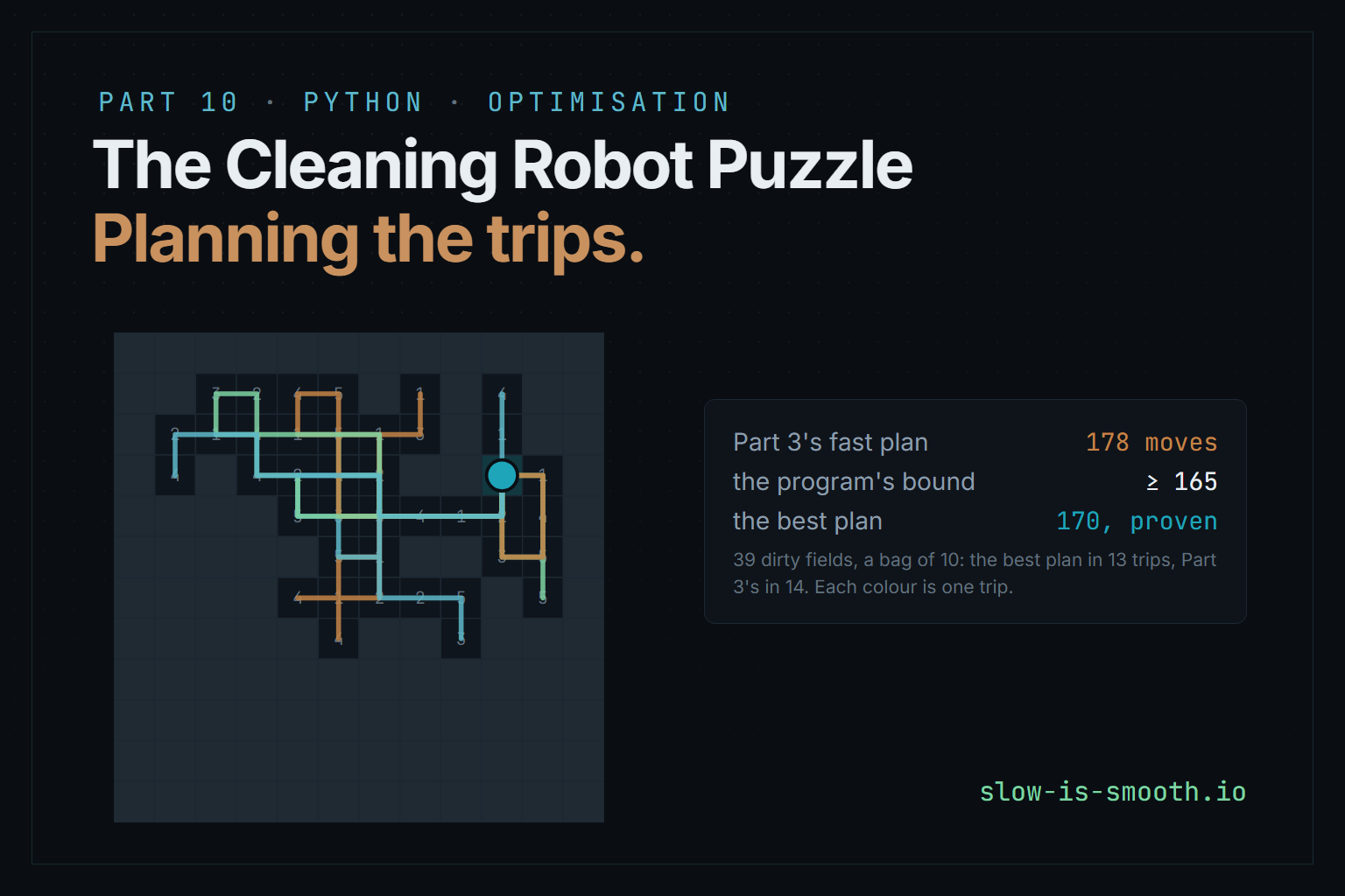
Part 3’s fast plan empties the robot’s bag on a furnished 12×12 room in 178 moves. The best plan takes 170, and this part proves that no plan takes fewer.
This is Part 10 of the cleaning robot puzzle. Part 3 gave the robot a small bag and a dock that empties it, and asked for the fewest moves that clean every dirty field. Its fast solver cuts one long tour into trips; its exact search tries every (field, cleaned fields, load) state and gives up beyond about nine dirty fields. Parts 8 and 9 wrote a route as numbers on pairs of fields. Here that model would need a whole copy of the room for every trip, so this part writes a plan the way the people who route real delivery vans do: as a choice among trips. There are more possible trips than atoms in the universe; the method below looks at a few hundred of them and still proves the answer. The new algorithms:
- a set-covering model over trips, whose linear program is far stronger than it looks;
- column generation: start with a handful of trips and let the program’s dual prices on the fields say which new trip is worth adding;
- pricing by labels and dominance: the cheapest trip under those prices, as a shortest path with the bag as a resource, and ng-routes, the relaxation that makes it fast;
- a completion bound by dynamic programming over (field, room left in the bag);
- reduced-cost enumeration: list every trip that could still be in a better plan, and solve over those, which turns the bound into a proof.
| File | What it does |
|---|---|
column_gen.py | the model, column generation, pricing, the completion bound, enumeration and the plans |
simplex.py | Part 8’s simplex method, as the from-scratch master program on small rooms |
test_column_gen.py | the checks and the report behind every number below |
Pricing, the completion bound and the enumeration are written from scratch; the master program runs on Part 8’s exact simplex method for small rooms and on HiGHS, through highspy, for the rest, and HiGHS solves the final integer programs. Every file behind all the parts is listed in the code’s README.
The problem again
Every floor field holds 1 to 5 units of dirt. The bag holds at most the capacity, and the dock, where the robot starts, empties it. The robot must clean every field and may finish anywhere. This part takes Part 2’s pick-cells rule: the robot drives with its brushes up and cleans a field with C, so it can cross dirty fields freely, and a trip is simply the list of fields it cleans, in order, walking the shortest way between them. Its cost is the moves: from the dock through the list and back, or, for the last trip, not back.
Part 3’s other rule, take all, cleans every field the robot drives onto. That makes a trip’s cost depend on which fields its walk crosses, not just which it cleans, and it breaks the model below; the end of this part says why.
A plan as a choice of trips
Number every possible trip : a list of fields whose dirt fits in the bag, closed or open. Let be its moves and if the plan uses it. Then
Every field is cleaned by some trip, and exactly one trip is the open last one. Asking for “at least once” rather than “exactly once” loses nothing: a field in two trips can be dropped from one of them, and since the walking distances are shortest paths, skipping a stop never makes a trip longer.
The model is simple because the hard part is inside the numbers : each already includes the best way to walk its trip. Relax to fractions and the linear program only has to choose among trips, never to route them, which is why its bound is so strong. On Part 2’s running example it is within two moves of the best plan at every bag size, where Part 3’s bound was up to eight short.
The trouble is how many trips there are. With 39 dirty fields and a bag of 10, a trip can clean up to 10 of them, in any order: far more trips than any program can hold.
Column generation
The way round it is to write the program with only a few trips, its columns, and add more only when they would help. Which would help is something the program itself can say.
Solve the linear program over the trips so far. Its dual solution puts a price on every field, the amount the cost would rise if that field had to be covered once more, and a price on the open-trip row. A trip not yet in the program is worth adding only if it costs less than the prices of what it does:
is its reduced cost, the same quantity the simplex method looks at when it picks a variable to bring in. If some trip has a negative one, add it and solve again. If none has, the current solution is optimal over every trip there is, and its value is a lower bound on every plan. column_gen.generate starts with every field on a trip of its own, closed and open, and loops:
for rounds in range(1, max_rounds + 1):
    value, pi, sigma, _ = master.solve()
    new = price(inst, pi, sigma)
    if record:
        record(rounds, value, pi, sigma, new)
    if not new:
        return value, master, rounds, inst
    for _, trip, open_ in new:
        master.add(trip, open_)
Column generation, round by round
Part 2's room with a bag of 23. Copper numbers are the program's price on each field; lines are the trips pricing found worth adding, in the order they clean.
The prices are the heart of it. At first the only trips clean one field each, so the prices are high; trips that clean several fields then look cheap, pricing adds them, and the prices fall. When they settle, a field’s price is its fair share of the moves in the best fractional plan. On the example the program needs 7 rounds and ends at 50/3, so no plan takes fewer than 17 moves.
Pricing: the cheapest trip under the prices
Pricing asks for the trip with the most negative reduced cost. Walking from field to field and cleaning it changes the reduced cost by , so it is a shortest path from the dock with those lengths, some of them negative, subject to two rules: the dirt must fit in the bag, and no field may be cleaned twice. That is the elementary shortest path problem with a resource constraint, and it is NP-hard: with negative lengths, “no field twice” is the Hamiltonian path problem again.
column_gen.price builds trips as labels, (last field, load, fields remembered, reduced cost so far), and extends each by one field at a time. What keeps the number of labels down is dominance: a label can be thrown away when another at the same field has no more load, no more reduced cost and remembers no field it doesn’t, because anything the first can still become, the second can become at least as cheaply:
new = (j, load + inst.dirt[j], (memory & ng[j]) | 1 << j, red + d[last][j] - pi[j], trip + (j,))
keep, bucket = True, buckets[j]
for other in bucket:
    if other[1] <= new[1] and other[3] <= new[3] + EPS and other[2] & new[2] == other[2]:
        keep = False
        break
On a 12×12 room with 63 dirty fields, the first version, which remembered every field a trip had visited, did not finish a single round in ten minutes: two labels almost never remember the same fields, so almost nothing is dominated. The fix is the ng[j] above. A label remembers only the visits among the fields near where it is now, its ng-neighbourhood of 8 fields; far away it forgets, and may come back to a field it cleaned long ago. So pricing now searches ng-routes, a larger set than the real trips, and every round took a tenth of a second.
Is the bound still right? When no ng-route has a negative reduced cost, no real trip has one either, since every real trip is an ng-route; the prices are then feasible for the dual of the program over all real trips, and by weak duality its value is still a lower bound. Only one thing has to match: an ng-route that visits a field twice has that field’s price subtracted twice, so it must go into the program covering that field twice. The first version shortened such routes to their first visits before adding them, which removed exactly what made them attractive; pricing found them again, forty rounds running, and the loop never ended. Counting visits in the program the same way pricing counts them fixed it. (A route that revisits a field is still a real plan, only a wasteful one: the robot drives over a field it has already cleaned.)
From a bound to the best plan
Column generation ends with a bound, not a plan: its solution usually uses fractions of trips. The quick way to a plan is to solve the integer program over the trips it generated. That is called price and branch, and it is only a heuristic: the best plan may need a trip no round ever asked for. On the 12×12 room it finds 172 moves, better than Part 3’s 178, but not the best.
The exact way is to generate the trips the best plan could use. Any plan’s cost can be written as the bound plus the reduced costs of its trips plus terms that are never negative:
because every field is covered at least once and every price is non-negative. Every reduced cost is non-negative too, at the end of column generation. So a plan that beats the best plan known so far, the incumbent, can only use trips with . column_gen.enumerate_trips lists all of them, keeping the cheapest order of each set of fields, and the integer program over that list is exact.
Listing them is a search over partial trips, and a partial trip can be abandoned as soon as it can’t finish within the gap. How low can its reduced cost still go? column_gen.completion answers with a lower bound for every (field, room left in the bag), by dynamic programming over q-routes: fields may repeat, so the answer is never too high, and a table of numbers covers every question the search asks.
On the 12×12 room the bound is 164.6 and Part 3’s fast plan, the first incumbent, has 178; price and branch lowers it to 172, so every trip with a reduced cost up to 172 − 164.6 is listed: 26,222 of them. Solving over those gives 170, and since they include every trip any plan of 169 or fewer could use, 170 is the best.
The best plans
Part 2’s running example:
| Bag | Part 3’s fast plan | Part 3’s bound | The program’s bound | Best plan | Trips enumerated |
|---|---|---|---|---|---|
| 5 | 60 | 53 | 58 | 60 | 36 |
| 10 | 32 | 24 | 32 | 32 | none needed |
| 23 | 18 | 13 | 50/3 | 18 | 568 |
Part 3's plan and the best one, trip by trip
Random rooms with 30% furniture and dirt from 1 to 5:
| Rooms | Dirty fields (mean) | Part 3’s fast plan | Part 3’s bound | The program’s bound | Best plan | Proven | Part 3’s plan over the best | Time |
|---|---|---|---|---|---|---|---|---|
| 6 of 8×8, bag 10 | 24 | 85.3 | 63.2 | 81.1 | 83.2 | 6 of 6 | 2.2 | 4 s |
| 6 of 10×10, bag 5 | 34 | 301.0 | 261.0 | 296.0 | 297.7 | 6 of 6 | 3.3 | 1 s |
| 6 of 10×10, bag 10 | 28 | 100.8 | 76.3 | 96.9 | 99.5 | 6 of 6 | 1.3 | 4 s |
| 4 of 12×12, bag 5 | 64 | 622.8 | 553.2 | 609.0 | 610.8 | 4 of 4 | 12.0 | 2 s |
| 4 of 12×12, bag 10 | 47 | 296.8 | 247.2 | 284.8 | 292.2 | 2 of 4 | 4.5 | 99 s |
| 2 of 12×12, bag 20 | 50 | 155.5 | 100.0 | 136.9 | 147.0 | 0 of 2 | 8.5 | 123 s |
Part 3’s fast plans are good, 1 to 12 moves over the best on average, and on every room its bound is far weaker than the program’s: on the 12×12 rooms with a bag of 20, Part 3 could prove 100 moves and the program 136.9. Where the method stops is where the gap between the bound and the best plan found stays wide, because the number of trips within the gap grows very fast with it and with the size of the bag: past half a million, the enumeration gives up. That happened on two of the four 12×12 rooms with a bag of 10, which end 2.6% and 3.3% from proven, and on both with a bag of 20, at 4.2% and 10.7%. A bigger bag means longer trips and many more of them. Closing those gaps is what the cuts of branch, cut and price are for: they raise the bound until the list of trips is short again.
Why take all doesn’t fit
Under Part 2’s other rule, the robot cleans every field it drives onto, and it may only drive onto a field whose dirt still fits. A trip is then no longer a list of fields to clean: the walk between them collects everything it crosses, and it may have to go the long way round a field that would overflow the bag. Its cost depends on the order and on the load at every step, and two trips can’t be priced independently, because what one cleans changes where the next may walk. The covering model assumes that a trip’s cost is fixed by the fields it cleans, and here it isn’t. Part 3’s take-all solvers stay the answer for that rule.
Testing Part 10
test_column_gen.py produces every number above:
| Check | How |
|---|---|
| Pricing | 150 random price vectors on tiny rooms, against every trip there is: with neighbourhoods covering the room the labels find the best trip; with neighbourhoods of two fields, never a dearer one |
| Completion and enumeration | 60 tiny rooms: the completion bound never overestimates the cheapest finish of any partial trip, and enumeration finds exactly the trips within the gap |
| The masters | 20 tiny rooms: the exact simplex method and HiGHS reach the same bound |
| Tiny rooms | 120 rooms: proven best, equal to Part 3’s trip oracle and its exact search, every plan replayed by Part 3’s simulator |
| The figures | docs/check_or_figures.py reruns the column generation and replays both plans, in Chromium |
What Part 10 teaches
- Choose the variables that make the bound strong. A plan as a choice of trips hides the routing inside each column’s cost, and the linear program only has to choose.
- Let the prices ask. Column generation never lists the trips; the dual prices say which one is missing.
- A relaxation that is easy to price can still prove things. ng-routes are not real trips, but if none of them helps, no real trip does.
- Count the same way on both sides. Pricing and the program must agree on what a column is, or the loop never ends.
- A good bound turns a search into a list. With the gap small, every trip that could matter can be written down, and the best plan is proven.