The magic number that was right for exactly one grid size
 The magic number that was right for exactly one grid size
Contents
In February a pressure solver in my CFD library stopped converging on a 33×33 grid. Within a day and a half every pressure solve had moved to a different algorithm, the iteration cap had gone up fivefold, two test grids had shrunk from 32 points a side to 9, and the old solver had been filed as legacy. A month later a pull request named the culprit: a relaxation factor hard-coded to 1.5. I went back and measured it. The number was within one sweep of the best on exactly one grid size, February’s failure turned out to have a different cause, and the formula that replaced the constant assumed walls the library does not have.
A Poisson solver, one tuning constant, forty-eight hours of commits, and what measuring every grid at every value of that constant says about each of them.
This post takes the story apart in the order it happened, and then puts the solver back together. Along the way it explains the method from scratch: what relaxation is, why a relaxation factor has a best value, why that value moves with the grid, and why missing it by a little costs a lot. Measuring the fix also turned up three bugs no test could see, one of which had been reporting diverged solves as converged. They are all fixed in the pull request this post was written alongside.
How to read this. Wherever you see a Predict box, stop and answer it before reading on. Several of the results here are not what the commit history, or I, expected, and the point is the gap between the guess and the measurement.
What you need to know already: some C, and what a grid of numbers is. The partial differential equation, the iterative methods and the theory behind the best relaxation factor are all explained where they first matter.
1. The failure, as the commits tell it
Here is what the repository recorded, in the words of its own commit messages. Times are as the commits record them, in UTC+2.
| When | Commit | What changed | What the message said |
|---|---|---|---|
| 7 Feb, 08:11 | b1a5b67 | The CPU projection solver’s pressure solve moves to conjugate gradients (CG) | “Switch CPU projection to CG_SCALAR for reliable convergence” |
| 7 Feb, 19:46 | be356a3 | The OpenMP projection solver moves to CG | “The OMP Red-Black SOR Poisson solver fails to converge on certain problem configurations (33x33 grids, small time steps)” |
| 8 Feb, 07:37 | 6a1c446 | Every Poisson solver’s default iteration cap goes from 1,000 to 5,000 | “Does not affect SOR/Red-Black solvers (they converge faster)” |
| 8 Feb, 13:13 | 0a64f2e | The SIMD projection solver moves to CG | “Red-Black SOR failed to converge within max_iterations on 32x32 and 64x64 grids” |
| 8 Feb, 13:54 | c2b2b67 | A Red-Black SOR test grid shrinks from 32×32 to 13×13 | “Red-Black SOR has O(n^2) iteration complexity vs CG’s O(n)” and “Red-Black SOR is a legacy solver” |
| 8 Feb, 14:00 | 05e510a | The same grid shrinks to 9×9, the cap rises to 50,000 and the tolerance is relaxed tenfold | “Even 13×13 grid failed to converge in CI.” |
| 8 Feb, 15:29 | 9811078 | The test’s right-hand side changes from a constant to zero | “uniform RHS which violates Neumann BC compatibility condition” |
| 7 Mar | #173 | SOR and Red-Black SOR compute their relaxation factor from the grid | “Hard-coded omega=1.5 was suboptimal for larger grids, causing Red-Black SOR to fail convergence on 33x33 grids within 1000 iterations” |
Read top to bottom, it is a tidy story. A solver fails on a bigger grid; it gets replaced where it matters, its tests get smaller until they pass, and a month later someone finds the root cause, a constant tuned for small grids.
Three details in that table do not fit the story, and this post is mostly about them. The commit that switched the OpenMP solver to CG also records, in its own root-cause list, that “GhiaProjectionAvx2Test (SIMD Red-Black) - PASSED”: a second implementation of the same algorithm with the same constant passed the same test on the same day. The test that kept shrinking was fixed, in the end, by changing its right-hand side and not its grid. And “O(n²) vs O(n)” is a claim about an algorithm that, as section 6 shows, describes the constant rather than the method.
To see why, we need to know what the solver was doing.
2. What the solver is for
The library simulates incompressible flow. Every time step it moves the velocity field forward ignoring pressure, and then corrects it so that no fluid appears or disappears. That correction needs the pressure , and the pressure comes from a Poisson equation,
where is built from how far the uncorrected velocity is from conserving mass. This is the pressure solve, and a projection solver does one every step, so it dominates the cost.
On a grid of points spaced apart, the Laplacian at a point is the sum of its four neighbours minus four times itself, divided by :
Solve that for the middle point and you get the sentence the rest of this post leans on: each value should be the average of its four neighbours, less a small correction from the right-hand side.
The border of the grid is the wall, and what the wall does matters more than you would think:
- Walls held at a value (Dirichlet walls). The border points are fixed, say at zero. There is exactly one solution.
- Walls with zero gradient (Neumann walls), which is what pressure at a solid wall gets and what the library does by default. After each pass, each border point copies the interior point next to it, so nothing changes across the wall. Now adding a constant to every changes nothing, so the solution is only defined up to that constant, and a solution exists only if sums to zero over the interior. Section 7 is about what happens when it does not.
A sweep is one pass over every interior point. The library measures progress with the residual, the largest amount by which any point misses its equation, and by default stops when the residual is a million times smaller than it was at the start.
3. Relaxation, from scratch
The averaging sentence suggests an algorithm straight away: start from a guess, replace every value with the average of its neighbours, and repeat. There are three classic ways to do the replacing.
Jacobi computes every new value from the old ones, all at once. It is trivially parallel and slow.
Gauss–Seidel walks the grid in order and uses each new value as soon as it exists, so the point to the right already sees the updated point to its left. It converges about twice as fast as Jacobi.
Successive over-relaxation (SOR) is Gauss–Seidel that overshoots. Gauss–Seidel says “move this point to the average”; SOR says “move it times as far”:
where is the Gauss–Seidel value. At it is Gauss–Seidel. Between 1 and 2 it over-relaxes, and for this kind of problem it converges for any strictly between 0 and 2. The relaxation factor is the constant this post is named after.
Red-Black SOR colours the grid like a checkerboard. A red point’s four neighbours are all black, so every red point can be updated at once, and then every black point. That makes SOR parallel, which is why the library’s OpenMP, SIMD and GPU solvers use it, and it converges at the same rate as the row-by-row version.
The figure below runs all three on the smallest problem that shows what they do: one row of points with both ends held at zero and no source, so the right answer is a flat line and everything you see is error.
Relaxing one row of points
Both ends are held at zero and there is no source, so the right answer is a flat line and everything you see is error. A toy with 15 unknowns, computed in your browser.
Before you look: the row starts as a broad hump with a ripple on top. After five Gauss-Seidel sweeps, which of the two is mostly gone?
Gauss-Seidel flattens the ripple within a few sweeps and hardly dents the hump: a point only learns about the far end of the rod one neighbour at a time. SOR over-steps every update; raise ω and the hump goes quicker, until past the best value the whole row starts to swing. A toy, computed in your browser, not the library.
Two things are worth taking from it. Relaxation kills short, jagged error almost at once and long, smooth error very slowly, because a point only learns about the far end of the grid one neighbour per update. And over-relaxing helps exactly with the smooth error, up to a point: raise too far and the whole row starts to swing.
4. Why there is a best ω, and why missing low costs more
In 1950 David Young worked out SOR’s convergence exactly for a class of matrices that includes this one. Call the factor by which the slowest error shrinks per sweep. Young showed that, with the Jacobi spectral radius from the box above, below a threshold
and above it
The threshold is where the square root reaches zero, and it is the best relaxation factor,
where drops to . For walls held at zero on a square grid, and this becomes the textbook . Because depends on the grid, so does the best : 1.674 on a 17×17 grid, 1.821 on 33×33 and 1.906 on 65×65. A constant can match that formula on one grid size at most.
The shape of is the other half of the story. Left of the optimum the curve plunges into it with an infinitely steep slope; right of it, it climbs back along a straight line of slope 1. So near the optimum, a step short costs more than the same step long.
This is a place where theory and a real library can be checked against each other directly. The figure draws Young’s curve from nothing but the grid size, and puts on it the rate the library’s own solvers actually achieved, measured over the second half of each run.
Predict. On a 33×33 grid the best ω is close to 1.82. Which takes more sweeps: 1.77, just below it, or 1.87, just above?
The kink at the best ω
How much one sweep shrinks the error, against ω, with walls held at zero. The line is Young's theory, worked out from the grid size alone; the dots are the library, measured.
Before you look: on a 33×33 grid the best ω is close to 1.82. Which takes more sweeps: ω = 1.77, just below it, or ω = 1.87, just above?
Below the best ω the measured dots sit on the curve; at and just above it the run is too short for the slowest error to take over, so a dot can land a little off. Sweeps are the library's own counts to a residual a million times smaller; “predicted” is the number of sweeps at the theory's rate.
Below the optimum the dots are not near the curve, they are on it: at ω = 1.5 on 33×33, Red-Black SOR shrank its residual by 0.970887 per sweep, and Young’s formula gives 0.970887. That is the whole theory confirmed, and it is also a warning. The formula is exact for the matrix it assumes. Section 10 is about what happens when the library’s matrix is not that one.
5. Predict, then measure
With the theory in hand, the February question is concrete: how far from the best was ω = 1.5?
To answer it I wrote a harness against the library’s public API at commit 9aa06d1, the last commit before this work, and ran Red-Black SOR and SOR at every ω from 1.00 to 1.99 in steps of 0.01 on grids from 9×9 to 129×129, then in steps of 0.001 around each minimum, with narrower scans on every grid from 5×5 to 17×17 and on 257×257. Every run solves the same problem: a pseudo-random right-hand side from a fixed seed, with its mean removed so the zero-gradient walls have a solution, from a zero start, to the library’s default tolerance. Every sweep count was replayed one sweep at a time through the library’s iterate call and matched.
Predict. On a 33×33 grid, with the walls the library had in February, how many times as many sweeps as the best ω does ω = 1.5 take?
Sweeps against ω, measured
The library's Red-Black SOR and SOR solving one problem at every ω from 1.00 to 1.99. The sweep axis is logarithmic: each gridline is ten times the one below.
Before you look: on a 33×33 grid, with the walls the library had in February, how many times as many sweeps as the best ω does ω = 1.5 take?
Measured, not simulated: the library's solvers on a seeded-noise right-hand side with zero mean, from a zero start, to a residual a million times smaller. “Before” is CFD at 9aa06d1, whose default walls are copied from the interior after each sweep; “relaxed at the wall” is the fix. The automatic ω is the library's own choice: the textbook formula before the fix, its estimate of the walls' optimum after it.
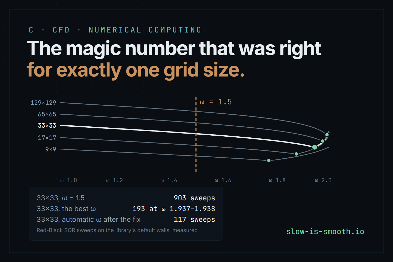
On 33×33, ω = 1.5 takes 903 sweeps and the best ω takes 193, 4.7 times fewer, and on 129×129 the gap is 14.7 times. Switch to walls held at zero and the curves drop and the minima move left, but from 17×17 up 1.5 is still far from the bottom: on 33×33 it takes 398 sweeps where the best takes 77.
The title claim deserves its own figure. Here is where the best ω falls on every grid measured, against the textbook formula.
Predict. With walls held at zero, SOR was measured on every grid from 5×5 to 17×17 and on four larger ones. On how many of those 17 is ω = 1.5 within one sweep of the best?
Where the best ω falls
The measured best relaxation factor on each grid, against the two formulas. The copper line is ω = 1.5.
Before you look: with walls held at zero, SOR was measured on every grid from 5×5 to 17×17 and on four larger ones. On how many of them is ω = 1.5 within one sweep of the best?
Measured with the library's solvers on one seeded-noise problem; each best ω is where a scan found the fewest sweeps, drawn as a short bar where several ω tied. The curves are formulas, computed in your browser.
With walls held at zero, ω = 1.5 is within a sweep of the best on exactly one grid, 10×10, which is where the textbook formula gives 1.490. With the zero-gradient walls the library actually uses, it is within a sweep of the best on none of the 25 grids and methods measured: the best ω for those walls sits far above the formula, above 1.7 even on a 5×5 grid. Keep that last observation in mind; it is the thread that leads to the real bug.
6. The constant changed the complexity class
Now back to “Red-Black SOR has O(n²) iteration complexity vs CG’s O(n)”. Here n is the number of points along one side, so the claim is that doubling the grid’s side quadruples SOR’s sweeps but only doubles CG’s.
Predict. With the library’s default walls, the grid goes from 129×129 to 257×257. At ω = 1.5, how many times as many sweeps does Red-Black SOR need?
Sweeps against grid size, measured
Each step to the right doubles the grid's side. Both axes are logarithmic, so a line's slope is how fast its sweeps grow: slope 1 doubles them with every doubling of the grid, slope 2 quadruples them.
Before you look: with the library's default walls, the grid goes from 129×129 to 257×257. At ω = 1.5, how many times as many sweeps does Red-Black SOR need?
Measured with the library's solvers on one seeded-noise problem, to a residual a million times smaller than it started. Slopes are fitted from 33×33 up. With the default walls, “before” is CFD at 9aa06d1 and “after” is the fix; walls held at zero are unchanged by it. CG is drawn only for walls held at zero.
At ω = 1.5, Red-Black SOR goes from 11,746 sweeps to 42,831, 3.6 times as many, and on log-log axes its line has a slope of 1.86. At the automatic ω of the fixed library it goes from 477 to 955, 2.0 times, slope 1.01. CG, with walls held at zero, has slope 0.98.
So the commit message measured something real, but it attributed it to the wrong thing. SOR at a fixed ω below the optimum is an O(n²) iteration; SOR at its optimum is O(n), the same class as CG. The constant 1.5 turned an O(n) method into an O(n²) one, and “legacy” was a judgement on the constant. At 257×257 the difference is 44.8 times the sweeps.
That does not make SOR better than CG, whose constant is smaller, or than the multigrid solvers the library also has. But it does mean the February decision to call Red-Black SOR legacy rested on a measurement of a misconfiguration.
7. Same weekend, different bug, same exit code
The test that shrank from 32×32 to 13×13 to 9×9 failed each time with the same code, -7. In this library
that is CFD_ERROR_MAX_ITER: the solver hit its cap. Each shrink looked like evidence that SOR is slow on
bigger grids, so the next step was a smaller grid, a larger cap and a looser tolerance.
It was not slow. The test gave the solver a uniform right-hand side with zero-gradient walls, and as section 2 said, those walls only admit a solution when the right-hand side sums to zero. A uniform right-hand side sums to anything but. There was no answer to converge to, at any grid size, at any ω, with any cap.
The fix that finally made the test pass, 9811078, changed the
right-hand side to zero, and its message names the compatibility condition correctly. But a zero right-hand
side from a zero start is already solved, so the test then passed after zero sweeps and tested nothing,
which is one of the loose ends in section 12. Two different failures, one from the constant and one from an
impossible problem, had printed the same -7 on the same weekend, and the second one had been read as more
evidence for the first.
8. Back to February
Which of the two broke the projection test on 7 February? The commit history cannot say, so I rebuilt the
library at 554a988, the parent of the commit that switched to
CG, added a log line to every pressure solve, and ran the test that failed, GhiaProjectionOmpTest, under four
variations. Each run makes 5,000 pressure solves on a 33×33 grid.
| Variation | Solves that converged | Solves that hit the 1,000 cap | Median sweeps when converged |
|---|---|---|---|
| As it was, ω = 1.5 | 1 | 4,999 | 717 |
| The textbook formula’s ω | 1 | 4,999 | 294 |
| ω = 1.5, right-hand side mean removed | 5,000 | 0 | 761 |
| The formula’s ω, mean removed | 5,000 | 0 | 298 |
Changing ω changed nothing: 4,999 solves capped either way. Removing the mean of the right-hand side fixed every one of them, at either ω. The projection step builds its right-hand side from the velocity field and never removed its mean, and on that test the mean was about 274,000 times the tolerance: every one of those capped solves was an impossible problem, the same bug as section 7 in production code.
Two more observations complete the picture, and one of them is a limit on what I can claim. The AVX2 build of the same test, the one the commit message said passed, logged exactly the same 4,999 capped solves, and so did the OpenMP build on 1, 2 and 8 threads, byte for byte. And on my machine the test’s final accuracy check passed in every variation, capped solves and all, with an RMS velocity error of 0.039. What reproduces is the capped solves the commit describes, not the red test on the CI runner that day. Whatever tipped that run over, it was not the choice of ω, and it was not a difference between the two builds. And the CG solver the commits switched to “converged” on all 5,000, by its own stopping test, while the zero-gradient residual SOR measures stayed above the tolerance on all 5,000 of them. CG did not fix the problem; it stopped reporting it.
So the attribution in #173 was wrong. ω = 1.5 did make every solve slower, by the margins in section 5, but it is not what failed that test.
9. The March fix, and what its test could not catch
The March pull request replaced the constant with the textbook formula, generalised for rectangular and 3D grids, and computed it at initialisation. Users can still pass an explicit ω, and zero, the new default, means “work it out”. That is the right design, and it made every solve faster than 1.5 did: on 33×33, Red-Black SOR went from 903 sweeps to 361.
Its test checked that Red-Black SOR on a 33×33 grid converges in fewer than 500 sweeps with the automatic ω, “the configuration that previously failed with omega=1.5”. On that test’s problem, ω = 1.5 takes 212 sweeps. The test would have passed before the fix. It could not have caught the premise being wrong, and it could not have noticed that 361 sweeps was still nearly twice the 193 the best ω achieves on the library’s walls, because nothing in it looked at the best ω.
That gap is the last clue. The formula is exact for walls held at zero, and the library’s walls are not held at zero.
10. The formula assumed walls the library does not have
Young’s result needs the iteration’s matrix to have a property called consistent ordering, which the five-point stencil with walls held at zero has. The question is whether the library’s zero-gradient walls keep it.
Look at what the default walls do. The sweep updates the interior; then each wall point is set equal to its interior neighbour. So during a sweep, a point next to a wall reads the wall’s value, and the wall’s value is a copy of that same point from before the sweep. The point is reading its own old value. That turns one of its four neighbours into a delayed copy of itself, and a matrix whose points depend on their own past values is not consistently ordered. Young’s formula, textbook or not, no longer describes the iteration.
I checked this without the library: building the exact iteration matrix of the library’s sweep, walls and all, and finding its best ω by computing eigenvalues. On 33×33 that best ω is 1.933. The formula gives 1.821. The measured best in section 5 was 1.937 to 1.938.
The fix changes one thing, only for the default walls. A point next to a wall relaxes against its real neighbours: its step is scaled by , where is the full diagonal and is the weight of its wall neighbours. That is 4/3 beside an edge and 2 in a corner, on a square grid. This makes the sweep exactly SOR on the zero-gradient matrix itself, which is consistently ordered, so Young applies again. The automatic ω becomes that matrix’s optimum as estimated at initialisation from a Rayleigh quotient of its slowest mode. A Rayleigh quotient can only overestimate that mode’s eigenvalue, so the estimate lands at or just below the optimum: 1.8633 on 33×33, against an exact optimum of 1.86331.
Here are the same curves as section 5, before and after.
Sweeps against ω, measured
The library's Red-Black SOR and SOR solving one problem at every ω from 1.00 to 1.99. The sweep axis is logarithmic: each gridline is ten times the one below.
Before you look: on a 33×33 grid, with the walls the library had in February, how many times as many sweeps as the best ω does ω = 1.5 take?
Measured, not simulated: the library's solvers on a seeded-noise right-hand side with zero mean, from a zero start, to a residual a million times smaller. “Before” is CFD at 9aa06d1, whose default walls are copied from the interior after each sweep; “relaxed at the wall” is the fix. The automatic ω is the library's own choice: the textbook formula before the fix, its estimate of the walls' optimum after it.
| Grid | Red-Black SOR, before | after | fewest after | SOR, before | after | fewest after |
|---|---|---|---|---|---|---|
| 9×9 | 76 | 25 | 21 | 77 | 28 | 24 |
| 17×17 | 162 | 54 | 49 | 150 | 61 | 56 |
| 33×33 | 361 | 117 | 104 | 380 | 135 | 120 |
| 65×65 | 709 | 235 | 221 | 751 | 268 | 246 |
| 129×129 | 1,451 | 477 | 447 | 1,473 | 521 | 504 |
| 257×257 | 2,885 | 955 | 892 | 2,732 | 1,021 | 1,021 |
“Before” is 9aa06d1 at its automatic ω; “after” is the fixed library at its automatic ω; “fewest” is the minimum over the scans on the fixed library. Solves take about a third of the sweeps they did, on every backend: the OpenMP and AVX2 Red-Black solvers match the scalar counts exactly, and the CUDA solvers, which check convergence every 20 sweeps, go from 360 to 120 on 33×33.
Two things in that table are findings rather than results.
The automatic ω is not quite the fewest sweeps. From 17×17 up it takes 0 to 13% more than the best scanned ω, and 17 to 19% more on 9×9. Little of that is the estimate falling short. On 9×9 it sits 0.0013 below the exact optimum, which accounts for one of the four extra sweeps; on 17×17 the gap is 0.0002 and on 33×33 0.00003, both inside one step of the scan. The rest is the optimum itself. At exactly the SOR iteration matrix is defective, its two slowest eigenvalues merge, and the error decays like instead of , so a solve converges slightly faster just above the optimum than at it. The textbook formula shows the same gap with walls held at zero, up to 21% on 257×257. A margin fitted to the data would close it, but it would be a tuned constant, the exact thing this story is about, so the library aims at the optimum and the tests allow 25%.
The walls now have a contract. Relaxing a wall point against its real neighbours only works if the wall is the default copy. Code that wrote its own wall values between iterations, instead of installing them through the solver’s boundary-condition hook, used to get away with it; now the corner factor, 2ω, passes 2, and it diverges. The library’s own accuracy test did exactly that and was fixed. The CUDA solvers apply the walls on the device and never call the hook, so they now refuse one instead of quietly solving with the default walls. The contract is documented where the hook is declared.
11. Three dimensions
The March fix extended the formula to 3D, and the same wall problem is there with six neighbours instead of four. On a 17×17×17 grid, Red-Black SOR at the automatic ω went from 225 sweeps to 64, with the fewest at 60. On a 33×33×9 slab it went from 1,099 to 140, fewest 127: the old 3D formula gave 1.616 for that grid, far below where the zero-gradient walls put the optimum, so it was the worst case in the whole study.
The wall factor generalises directly, a corner in 3D has three wall neighbours, and the Rayleigh quotient takes the slowest mode along each axis and keeps the smallest.
12. Loose ends found while measuring
Measuring every backend before and after the fix turned up problems no existing test could see. Each is fixed in the same pull request, with a test that fails on the old code.
A diverged solve could report convergence. The residual was computed as a running maximum with >. A
NaN compares false against everything, so once a field overflowed, every NaN residual was skipped and the
maximum came out as zero, which is below any tolerance. The solve loop then reported success. The residual
now keeps a NaN, and the loop stops with a divergence status as soon as the residual is no longer finite.
The CUDA solvers, which run loops of their own, used to switch their checks off on such a residual and run out
the cap; they now stop as diverged too.
The AVX2 SOR solver always diverged. It used a Block SOR: four cells at a time, where the second, third and fourth cells of each block read their left neighbour from the previous sweep. That is not SOR, it is a different iteration, and on every grid measured, 17×17 to 65×65, it diverged once ω reached 1.45 or 1.50, below every one of those grids’ automatic ω. Combined with the NaN bug, it reported convergence every time: a 33×33 solve at the automatic ω “converged” after 1,764 sweeps with a residual of exactly zero. No test solved anything with it. It now computes, four cells at a time, only the stencil terms the sweep does not write, and then relaxes the row in order, which makes it the scalar SOR iteration sweep for sweep: 135 sweeps on 33×33, like the scalar solver.
Gauss–Seidel was SOR in disguise. The factory gave the Gauss–Seidel method the SOR solvers without marking them, so it ran at SOR’s automatic ω: 380 sweeps on 33×33 where ω = 1 takes 2,376. It now always runs at ω = 1.
Two tests tested nothing. The Red-Black SIMD tests that replaced the impossible uniform right-hand side with a zero one converged before their first sweep. They now solve a problem with an answer and compare the SIMD result to the scalar one.
The tuning example still recommended 1.5. The library’s own solver-comparison example benchmarked SOR at the old constant. It now uses the automatic ω.
One thing is recorded as a follow-up rather than fixed. The projection solvers still remove the mean of the pressure right-hand side only in one multigrid mode, so the February bug is still reachable if someone configures an SOR-family pressure solve.
13. The general shape
A tuning constant is a claim about the input. omega = 1.5 claimed a grid of about ten points a side with
walls held at zero, and the code was run on neither. The formula that replaced it made a better claim, about
every grid size, and still one about the walls. The pattern repeats all the way down this post: an exit code
that meant “cap reached” was read as “too slow”, a test that passed was read as covering the premise, and a
residual of zero was read as success.
What would have caught each of them is the same kind of evidence: sweep the parameter and look at the whole curve, not one point on it. A constant that is right should sit at the bottom of its curve on the inputs the code actually sees. If you cannot say where the bottom is, you cannot say the constant is right.
Run it yourself
The pull request adds an example that does exactly the sweep in section 5 on one grid, with any method, backend and walls, and prints CSV ending with the automatic ω’s row. Pinned at the merge commit:
git clone https://github.com/shaia/CFD.git && cd CFD
git checkout 23b196a
cmake -S . -B build -DCMAKE_BUILD_TYPE=Release -DBUILD_EXAMPLES=ON
cmake --build build --config Release --target sor_omega_sweep
./build/sor_omega_sweep --grid 33 --from 1.80 --to 1.95 --step 0.05
On the fixed library, built with MSVC, that prints (another compiler can differ in the last digits):
omega,sweeps,status,final_residual
1.8000,244,converged,9.639475e-07
1.8500,154,converged,9.741168e-07
1.9000,145,converged,9.315211e-07
1.9500,294,converged,6.763749e-07
auto,117,converged,9.625996e-07
With Visual Studio the program lands in build/Release/. --method sor switches to row-by-row SOR and
--walls dirichlet holds the walls at zero. --backend omp runs Red-Black SOR on OpenMP; --backend simd needs
the build configured with -DCFD_ENABLE_AVX2=ON on x86, and --backend gpu with -DCFD_ENABLE_CUDA=ON, and the
CUDA solvers take only the default walls. The example uses only the public API, so it also builds on the commit
before the merge: copy examples/sor_omega_sweep.c into that checkout, add the same two lines to
CMakeLists.txt, and the same command draws the “before” curve, ending with 361 sweeps at the automatic ω.
A note on the evidence
Every number in this post is measured or labelled as computed. The sweep counts come from a harness that calls the library’s public API, built with MSVC 19.44 in Release on an Intel i9-13980HX under Windows 11, at CFD 9aa06d1 for “before” and on the pull request’s branch for “after”. Rerun at the merge commit, 23b196a, the scalar “after” runs behind sections 6, 10 and 11 reproduced byte for byte. Each count was replayed sweep by sweep and matched. The per-backend comparison used the sweep example in a Debug build, and the GPU runs an RTX 4090 Laptop GPU with CUDA 13.0. The February reconstruction rebuilt 554a988 with a logging patch that is not in the repository.
The figures draw from the same recorded runs: each carries its data in its own source, written by a script from the run files, and each header records a Node replica that recomputed what the figure shows. The run files, the harness and the theory scripts are published with this post, starting from their README, and claims.csv maps every number in this post to its source.
Not verified locally: the NEON solvers, which the pull request’s CI runs on Apple Silicon, and builds with GCC and Clang, which it runs on Linux.