The 1.5× that three benchmarks tried to hide
 The 1.5× that three benchmarks tried to hide
Contents
Doing one step of a learned Bloom filter’s query four lanes at a time made it 1.5 times faster with the filter in cache, and three benchmarks along the way said otherwise. The first said the change made code it never touched 10% slower. The other two ran on a laptop that had quietly throttled, and said it made queries slower, at one size almost twice as slow. None of them was measuring the change. This is the step, the rounding argument that makes its answers exact, and how each of the three was caught.
Part 9 of the Bloom filter saga: an AVX2 score-to-region lookup for a partitioned learned Bloom filter, the test that catches a missing correction when every end-to-end test passes, and the benchmarks that lied about it.
Part 8 ported Sato and Matsui’s fast construction of a partitioned learned Bloom filter to C++, and left the search at about half a millisecond, a tenth of a build. What remains is what a filter is for: answering queries. This part follows one optimisation of the query path in the same port, learned-bloom-filter, from the measurement that suggested it to the measurements that nearly talked me out of it. Every number comes from that code; the files are named as we go, and the ones I could not keep are said to be so.
How to read this. Where you see a Predict box, stop and answer it before reading on. The three figures are interactive; the first computes everything it shows exactly as the library does, and the last draws only recorded measurements. The box marked “safe to skip” holds the derivation; the main text never depends on it.
What you need to know already: what a Bloom filter is and what a learned one adds, both covered at the start of Part 8. SIMD, gathers, prefetching and the rest are explained where they first matter.
1. What a query does
A query to a partitioned learned Bloom filter arrives as two numbers: the key’s 64-bit hash, and the score the classifier gave it, between 0 and 1. The filter then does two things. It finds the score’s region, the band of scores whose backup filter speaks for this key, and it asks that backup filter whether the key is present.
The second step is the familiar one, with a twist in how the filter is laid out. The Go filter at the start of this saga arranged its bits in 64-byte cache lines, but a key’s bits could fall in any of them, so a lookup touched up to one line per hash function, and the early parts of the saga spent much of their effort making those accesses cheaper. A blocked Bloom filter (Putze, Sanders and Singler, 2007) removes the problem at the source: it confines all of a key’s bits to one small block, so a lookup is one memory access. The port uses its tightest form, the split-block Bloom filter that Apache Parquet standardised for the per-column-chunk filters its readers use to skip data (the Parquet specification):
- A block is 256 bits, held as eight 32-bit words.
- The hash’s high 32 bits pick the block. Multiplying them by the number of blocks and keeping the top 32 bits of the product maps them evenly onto any block count, with no division.
- The hash’s low 32 bits pick one bit in each of the eight words: multiply them by a fixed odd constant, a different one per word, and keep the top five bits of the 32-bit product, a number from 0 to 31. The eight constants are Parquet’s, so a block built here means the same thing to any implementation of the spec.
- Inserting sets those eight bits. A query loads the 32-byte block once and checks all eight with one vector instruction.
The figure is a twelve-block filter you can fill. Its arithmetic is the library’s, checked against the C++ for a handful of keys before it went up.
One key, one block, one bit in each word
A twelve-block split-block filter. Insert keys 1, 2, 3, … and query non-keys counted up from 1,000,001; every hash, block and bit is computed the way the C++ library computes it.
Insert a few hundred keys and query a thousand non-keys, and the measured false-positive rate settles near the model’s prediction, the same Poisson sum the library uses to size every filter. The price of fitting each key into one block is memory. At a 1% rate a split-block filter needs 10.53 bits a key against a classic Bloom filter’s 9.59, about 10% more, and the gap widens at loose rates: at 50% it is 3.25 bits against 1.44. A learned filter has loose regions by design, so it pays more than a plain filter does, about a fifth over Part 8’s cost model rather than a tenth, which is the overhead Part 8 deferred to here. It buys a probe that costs the same whatever the region: one load and one test.
The first step, finding the region, is a chain of four small lookups:
- Score to segment. The build cut the score range into equal segments. The segment is
the smallest whose threshold is at least the score, exactly as the Python
reference’s
bisect_leftdecides it, ties included; Part 8 is about why “exactly” matters. - Segment to region, from a table of 1,002 small integers.
- Region to slice. Every region’s backup filter is a run of consecutive blocks in one shared array, and the region’s slice records where its run starts and how long it is.
- Slice and hash to block, by the multiply-and-keep-the-top step above, scaled to the slice.
Two regions are special. A region whose optimal false-positive rate came out as 1 needs no filter at all, and one at rate 0 would reject everything. Rather than branch on either, the port points them at two sentinel blocks at the front of the array, one of all ones and one of all zeros. Every query then runs the same load and test, whatever region it lands in, which matters for what follows: code that never branches on the data is code that can do four queries at once.
2. Where the time goes
The port answers queries in batches. It works through them 64 at a time: first it computes every query’s block address and issues a prefetch for it, a hint that asks the memory system to start fetching a cache line before it is needed; then it probes all 64. The misses overlap instead of queueing, and on a filter too big for the caches that is most of the win. On a filter that fits in the CPU’s L2 cache, the misses are cheap and the arithmetic shows through.
Here is one recorded run, with the filter at 200,000 keys: 178 KB, inside this laptop’s 2 MB L2. Half the queries are keys and half are unseen non-keys, in random order. A plain split-block filter at the same 1% target is there for scale; it has no regions, so it has no lookup.
| ns per query | |
|---|---|
learned filter, contains() one at a time | 11.52 |
| learned, batch, scalar lookup, scalar probe | 8.44 |
| learned, batch, scalar lookup, AVX2 probe | 4.53 |
| plain split-block filter, AVX2 batch | 1.19 |
Batching and an AVX2 probe have already done their work: 11.52 down to 4.53. But the plain filter, which probes the same kind of block in the same kind of batch, takes 1.19. The 3.3 nanoseconds between them is everything the learned filter does that a plain one does not, and that is the four-step lookup. It is three quarters of the query. The learned filter is 32% smaller (7.11 bits a key against 10.53) and meets the same target (a measured 0.99% against 1.00%), but in cache it is paying for that with the lookup.
The four steps are short and branch-free, except for one. Finding the segment computes , which in exact arithmetic would be the answer, and then corrects it with two loops, because the score and the thresholds are rounded doubles and the guess can be off near a threshold:
std::size_t index(double score) const noexcept {
    const std::size_t n = segments();
    if (!(score > 0.0)) return 1;  // also catches NaN
    if (score >= 1.0) return n;
    auto i = static_cast<std::size_t>(std::ceil(score * static_cast<double>(n)));
    if (i < 1) i = 1;
    if (i > n) i = n;
    while (i > 1 && thresholds_[i - 1] >= score) --i;
    while (i < n && thresholds_[i] < score) ++i;
    return i;
}
It reproduces the reference’s bisect_left exactly, which the golden tests demand. It is also a loop
whose trip count depends on the data, which is the one thing a four-lane version cannot have.
3. Four lanes, and one step each way
SIMD, single instruction, multiple data, is the CPU doing the same operation on several values at once. AVX2’s registers are 256 bits wide, room for four doubles, so one multiply computes for four scores and one rounding instruction takes all four ceilings. It also has gathers: one instruction that loads four values from four unrelated addresses, given a base pointer and four indices. With those, every step of the lookup can run on four queries together, except the correction loops.
So the question is how far the loops can go. If the rounded guess can be off by any amount, the vector code needs a loop with a lane mask, and most of the speed goes. If it can be off by at most one in each direction, the loops are one comparison each: gather the thresholds on either side of the guess, compare, and step.
Predict. The score and the thresholds are each within a rounding error of their exact values. With up to a million segments, how far can land from the true segment: one, two, or does it grow with ?
One, at any the library allows, and in only one direction for a given score. The figure walks through the three cases at , with two real scores where the guess is wrong:
Why one step each way is enough
N = 50 segments. The vector code guesses the segment as c = ceil(s × N), then checks the two stored thresholds next to the guess.
The middle case is the instructive one. The score 0.14000000000000001 is exactly the stored threshold , so it belongs to segment 7: segments include their top threshold. But has no exact binary form, and the stored double is a hair above the real . Multiplied by 50 it comes out a hair above 7, and the ceiling says 8. The guess is wrong not because the multiply rounded badly but because the boundary it assumes, the integer 7, is not where the stored threshold put it. The third case is the mirror image: the double just above belongs to segment 36, but its product with 50 rounds down to exactly 35. One gather of catches the first, one gather of the second.
That argument is the comment above the vector function in
segments.hpp,
and the function is nearly a transcription of it:
PLBF_TARGET_AVX2 __m128i index4_avx2(__m256d score) const noexcept {
    const __m256d n = _mm256_set1_pd(static_cast<double>(segments()));
    const __m256d one = _mm256_set1_pd(1.0);
    __m256d c = _mm256_ceil_pd(_mm256_mul_pd(score, n));
    c = _mm256_min_pd(_mm256_max_pd(c, one), n);
    const __m128i ci = _mm256_cvttpd_epi32(c);
    const double* t = thresholds_.data();
    const __m256d below = _mm256_i32gather_pd(t, _mm_sub_epi32(ci, _mm_set1_epi32(1)), 8);
    const __m256d at = _mm256_i32gather_pd(t, ci, 8);
    const __m256d down = _mm256_and_pd(_mm256_cmp_pd(below, score, _CMP_GE_OQ), one);
    const __m256d up = _mm256_and_pd(_mm256_cmp_pd(at, score, _CMP_LT_OQ), one);
    c = _mm256_add_pd(_mm256_sub_pd(c, down), up);
    // Only reachable outside (0, 1): down at c = 1 for s <= 0, up at c = N for s > 1.
    c = _mm256_min_pd(_mm256_max_pd(c, one), n);
    return _mm256_cvttpd_epi32(c);
}
The scalar version’s early returns become clamps. A score at or below 0 has its guess clamped to 1, and
a score at or above 1 to . NaN needs no case of its own: max_pd returns its second operand when
the first is NaN, which sends it to 1, and the ordered compares on a NaN are false, so it takes no
step. The final clamp only matters outside , where a correction can push past the ends.
The rest of the lookup is two more gathers and some integer arithmetic, in plan4_avx2 in
filter.hpp.
The region table holds 16-bit entries, and AVX2 has no 16-bit gather, so the code gathers 32 bits at
each entry’s address and masks off the top half. The read for the last segment would run one entry
past the table, so the table carries a pad entry for it. Each slice is packed into one 64-bit word,
the first block in the high half and the count in the low half, so a single 64-bit gather fetches both.
That layout earns its keep in the next instruction: _mm256_mul_epu32 multiplies the low 32 bits of
each 64-bit lane, which is exactly the hash’s high half (shifted down) by the slice’s count. The top
half of that product is the block within the slice; add the slice’s first block, multiply by 32 bytes,
add the array’s address, and prefetch all four.
Predict. The lookup was three quarters of an in-cache query, and now it does four queries per step. How much faster does the in-cache batch get: about 4×, about 2×, or less?
Less, and how much less depends on where the filter lives:
| filter | scalar lookup | AVX2 lookup | speedup | plain filter |
|---|---|---|---|---|
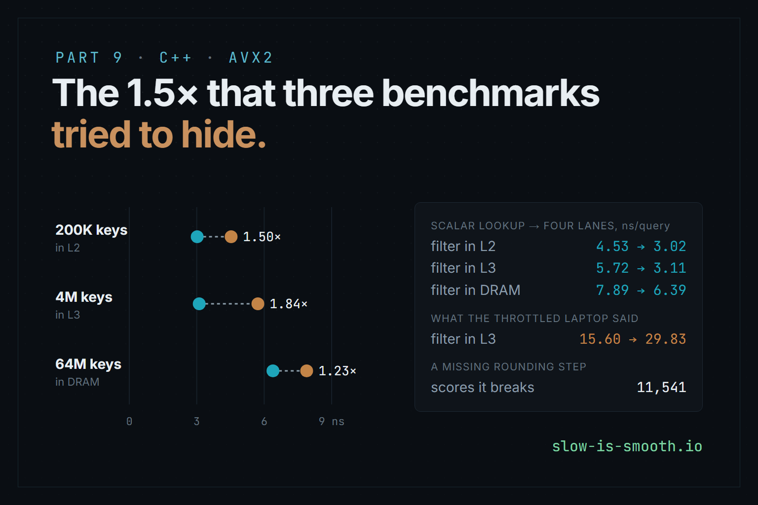
| 200,000 keys, 178 KB, in L2 | 4.53 ns | 3.02 ns | 1.50× | 1.19 ns |
| 4,000,000 keys, 3.4 MB, in L3 | 5.72 ns | 3.11 ns | 1.84× | 2.13 ns |
| 64,000,000 keys, 56 MB, in DRAM | 7.89 ns | 6.39 ns | 1.23× | 7.22 ns |
Both batches share the probe and the prefetch, and differ only in the lookup, so the difference is the lookup’s. Four lanes do not make it four times cheaper, because a gather still performs four loads; it only issues them as one instruction. What the vector version removes is the instructions around the loads, the branches, and the one-query-at-a-time dependency chain from score to address. In L2 the learned filter now costs about 1.8 nanoseconds a query more than a plain one, down from 3.3. In L3 the gain is larger still, though the lookup is a smaller share of the query there; the arithmetic is the same, so the difference must be in how the lookup overlaps the slower probes, and I have not measured that directly. Past the L3 cache, memory latency dominates everything and the lookup is a smaller part of the wait. There the learned filter’s batch is even faster than the plain filter’s, 6.39 against 7.22 nanoseconds. I have not taken that apart. The likely reasons are that it is a third smaller and that the queries landing in its sentinel regions never leave the cache, but that is unmeasured.
4. Testing it
The bound says one step each way. The test has to show the code takes that step at every score where it
could matter, and nowhere else. Random scores are almost useless for that, since a random double lands
within a few ulps of a threshold about never. So the test in
test_filter.cpp
builds its scores from the thresholds themselves:
- every threshold of the grid, and the doubles immediately below and above it;
- 0, −0, 1, −1, 2, the smallest subnormal and normal doubles, the doubles either side of 1, ±1e300, ±∞ and NaN;
- 100,000 uniformly random scores, for good measure.
It does that for ten grid sizes: 1, 2, 3, 7, 50, 1,000, 4,096, 65,537, 1,000,003 and 16,777,217. The odd sizes are there because with odd is never an exact binary fraction inside , and the large because the product carries the most rounding there. That is 54,543,918 scores, and on every one the four-lane index equals the scalar one.
A test that passes is only evidence if it could have failed, so I broke the code on purpose: I deleted
the downward step, the _mm256_sub_pd(c, down), and ran the suite again
(test_filter_mutant.txt).
segments: the four-lane index equals index() everywhere
  FAIL  54543918 scores over 10 grids, N up to 2^24 + 1  (11541 != 0)
It fails on 11,541 of the 54.5 million. That was the result I wanted. What I had not expected was
the rest of the output. Every other test in the suite still passed, including “every batch kernel
equals contains()”, which runs all three batch kernels against the one-at-a-time query on edge scores
and ragged batch lengths, and “no false negatives”, which queries every inserted key through every
kernel.
Predict. The mutant puts thousands of scores in the wrong segment. Why does a test comparing whole filter answers not notice?
Because a wrong segment rarely means a wrong answer. A segment maps to a region, and a filter with 9 regions over 997 segments has only 8 places where neighbouring segments belong to different regions. A misplaced score anywhere else lands in the right region anyway and gets the right answer. At the 8 boundaries a non-key is probed in the neighbouring region’s filter instead, which says “absent” too, almost always. And the keys in the no-false-negatives test have random scores, which never sit exactly on a threshold. So the end-to-end tests would have shipped this bug.
It is not a harmless bug. At the paper’s , it happens that no threshold inside ever needs the downward step, but at five do: 0.07, 0.14, 0.28, 0.55 and 0.56, as doubles. In floating point 0.07 × 100 is 7.000000000000001. Suppose a classifier rounds its scores to two decimals, and the build puts a region boundary after segment 7. Then every key that scored exactly 0.07 was inserted into the lower region, by the scalar code at build time. At query time the broken vector code would look it up in the region above, whose filter never saw it: a false negative, the one thing a Bloom filter promises never to give. Only a test at the level of the index, aimed at the thresholds, sees it coming. Dropping the upward step instead fails on 23,150 scores. The reducer in section 7 counts 23,190 upward steps; the other 40 are on scores of 1 or more, which the final clamp catches anyway.
5. Three benchmarks that said otherwise
The proof and the test say the four-lane lookup is exact. Whether it is faster is a separate claim, and the benchmarks on the way to the table above made it hard to establish. Three of them said something false, each for a different reason, and none of the reasons was the code.
The harness that slowed code it never touched
The first comparison I made, during development on 29 October, set the benchmark from before the change against the benchmark after it. The “after” benchmark had been rewritten too, to time the new kernel beside the old one. The vector lookup was clearly faster. But the scalar paths, which the change had barely touched, came out about 10% slower, one query at a time and in the scalar batch alike.
I went looking for what the change had done to them, and found two plausible suspects:
- The packed slice. To feed the 64-bit gather, the change had packed each region’s slice into one word, so the scalar path now unpacked it with a shift and a mask. I gave the scalar paths back their old two-field struct.
- The benchmark’s own loops. The new benchmark kept its variants as a list of lambdas, and the two
loops it wrote itself read the queries through the lambda’s captured references. A store through a
uint8_t*may alias anything, including those references, so the compiler must reload them on every iteration. I moved the reads into locals.
Neither closed the gap. With both suspects dealt with, five alternating runs of each benchmark still put the median one-at-a-time query at 9.75 nanoseconds before against 11.25 after, and the scalar batch at 7.69 against 8.35. What gave it away was a control. The plain split-block filter’s loop, whose code no part of the change had touched, had slowed down too, from 4.24 to 4.61 nanoseconds. A change cannot slow down code it does not contain, so the regression was in the benchmark binary, not the library.
The fix was not to explain the difference but to remove it. I compiled the old benchmark source against both the old headers and the new ones, so the two binaries differed only in the library, and ran them alternately, six times each, each binary alone. The scalar paths did not move: 9.96 against 9.97 nanoseconds one at a time, 8.16 against 8.03 for the scalar batch. The AVX2 batch went from 4.31 to 2.76, 1.56×. Under the same harness, the packed slice measured no slower than the struct either, so I went back to the single packed form. Why two builds of the same library code differed by 10% I never established. Code placement and different inlining decisions are the usual suspects, and the method that matters is the one that made the question unnecessary.
The second suspect, the aliasing reload, left one false number behind. While chasing the gap I wrote
in the benchmark’s source that reading through the captures costs “~0.9 ns/query, measured”. That 0.9
was the gap between the two harnesses, not a measurement of the reload, and it shipped in the
published code. So I measured it properly for this post
(captured_vs_locals.txt).
I built the benchmark twice, identical except for those two loops, and ran the builds alternately, six
times each, with the throttle probe described below on either side. The four variants that loop inside
the library are the controls, since they never see the change. The reload is real. Compiled on its
own, a minimal version of the loop shows it: g++ 16 at -O3 emits three loads per iteration that the
locals version hoists out of the loop.
.L20:                                   # reading through the closure
	mov	r9, QWORD PTR [rcx]             # the hashes' data pointer, again
	mov	r10, QWORD PTR [rdx]            # the output's data pointer, again
	mov	rbx, QWORD PTR [r9+rax*8]
	...
	mov	BYTE PTR [r10+rax], r9b
	add	rax, 1
	cmp	rax, QWORD PTR [r8]             # the count, again
	jb	.L20
But it costs 0.31 nanoseconds a query on the learned filter’s loop and 0.25 on the plain filter’s, a third of the claim. The controls moved by 0.09 or less. The comment now says so.
The laptop that changed speed mid-run
The second false benchmark was the first attempt to record the numbers for these posts, on 30 October. The table in section 3 has the 4-million-key result from the recorded run: 5.72 nanoseconds for the scalar lookup, 3.11 for the vector one. The first attempt, same binary, same filter, said 15.60 and 29.83, the vector lookup almost twice as slow.
What had happened was the laptop. Its power settings had put it in a mode that cuts the CPU’s power
within seconds of sustained load. To see it, I wrote a small probe,
throttle_probe.cpp,
that prints a single-thread compute rate and a memory-latency figure about twice a second. Within five
seconds of load its compute rate fell from about 1,190 to 160 million operations a second, and its
memory latency rose from 94 nanoseconds to as much as 200. Once that took hold, the benchmark’s CPU
figures came out 2.5 to 9.6 times too slow, the untouched plain filter included: its loop took 37.19
nanoseconds against a clean 8.72. The 200,000-key section, run before it took hold, was not slow at
all.
The benchmark reports the best of seven rounds, and that does not save it. A minimum over rounds is a
good estimate of what code costs on a steady machine, because noise only ever adds time. A machine
whose speed changes between rounds is not noisy; it is a different machine at different moments, and
the minimum just picks whichever variant happened to run in a fast one. What I cannot explain is that
the throttled runs were not random about it. In all seven degraded measurements I have at the two
larger sizes, two from this recording and five from development, the vector lookup came out slower
than the scalar one. Gathers may suffer more than ordinary loads when the core is starved of power, or
the interleaving may put one variant at a worse point in each cycle. I did not chase it, because the
remedy is the same either way: the throttled files are kept in
throttled/
as evidence of a failure, and quoted only here.
The runs past L3 that came out a wash
The third was during development, a day earlier, and it was the same failure arriving slowly. In the first clean run at 64 million keys, the vector lookup took 5.98 nanoseconds against 6.80 for the scalar one. Then the machine’s memory latency rose seven or eight times for every variant, the plain filter included. In each of four later runs at that size both lookups took between 37 and 53 nanoseconds, with the vector one behind every time, and the difference being measured, under a nanosecond, was lost in the drift. The laptop was in the same power mode, and changing system settings was not mine to do from a benchmark. So the port’s README said the DRAM result was inconclusive, and asked for a rerun on a quiet machine. That rerun is the 1.23× in the table. The probe either side of it shows a machine nowhere near the state of the throttled run. Before it, the probe’s compute rate held between 956 and 1,196 million operations a second. After it, the rate started above 1,000 and sagged to about 530 under the probe’s own sustained load, against 160 when throttled.
One speedup, two ways to mismeasure it
The figure puts the three kinds of evidence side by side. The result is one clean run at three sizes. The loop comparison is a harness effect isolated with controls that do not move. The throttled comparison is what a machine effect looks like: everything moves, unevenly.
6. A benchmark you can believe
None of this is new advice, but each item below is here because skipping it produced a wrong number in this one project:
- Change one thing. Compare two builds of the same benchmark source, or better, two code paths in
one binary. The port keeps the old lookup as
kernel::avx2_probefor exactly this reason: the recorded speedup is between two kernels in the same executable, under the same harness, in the same run. - Include controls. Time something the change cannot affect. If it moves, the measurement is measuring something else. The plain filter’s loop caught the harness; the plain filter’s batch caught the throttling.
- Alternate, and run alone. Interleave the variants, run each binary alone, and alternate the binaries, so slow drift lands on both sides. Across runs, report the median and the range, not the one best run.
- Watch the machine. A laptop’s power policy can change its speed by an order of magnitude a few seconds into a run, and the operating system may not say so: Windows reported the same power scheme throughout all of this. A probe before and after costs a minute.
- Compare within a run. This machine ran the same benchmark 10 to 25% slower on one day than the day before, and the loop comparison, recorded later on the same day as the table, came out about 20% faster than the table across the board. Every comparison in these posts is between numbers from one run, or from runs alternated in one sitting.
- Check the answers too. Every kernel has a test against the one-at-a-time query, and every benchmark variant prints its measured false-positive rate. A fast wrong answer shows up there before it shows up anywhere else.
7. Run it yourself
The figures and the tests are the library’s, which you would have to build. Here instead is the whole
argument in one file: the scalar index, the four-lane index with its two corrections, and the edge
scores, for the same ten grids. It counts how often each correction fires and how often the two indexes
disagree. Build it again with -DBROKEN to drop the downward step.
// The four-lane score-to-segment lookup, against the scalar loop it replaces,
// on every score where rounding could tell them apart. -DBROKEN drops the
// downward correction.
//   g++ -std=c++20 -O2 -mavx2 edges.cpp -o edges && ./edges
#include <immintrin.h>

#include <cmath>
#include <cstdint>
#include <cstdio>
#include <limits>
#include <vector>

struct Grid {
    std::vector<double> t;  // t[i] = i / N, correctly rounded: the segment thresholds
    explicit Grid(std::uint32_t n) : t(n + 1) {
        for (std::uint32_t i = 0; i <= n; ++i) t[i] = double(i) / n;
    }
    std::uint32_t n() const { return std::uint32_t(t.size() - 1); }

    // The smallest i >= 1 with t[i] >= s; out-of-range scores and NaN clamp.
    std::uint32_t index(double s) const {
        const std::uint32_t n = this->n();
        if (!(s > 0.0)) return 1;
        if (s >= 1.0) return n;
        std::uint32_t i = std::uint32_t(std::ceil(s * n));
        if (i < 1) i = 1;
        if (i > n) i = n;
        while (i > 1 && t[i - 1] >= s) --i;
        while (i < n && t[i] < s) ++i;
        return i;
    }

    // The same for four scores: c = ceil(s N), then one compare each way.
    __m128i index4(__m256d s, long& downs, long& ups) const {
        const __m256d n = _mm256_set1_pd(this->n()), one = _mm256_set1_pd(1.0);
        __m256d c = _mm256_ceil_pd(_mm256_mul_pd(s, n));
        c = _mm256_min_pd(_mm256_max_pd(c, one), n);
        const __m128i ci = _mm256_cvttpd_epi32(c);
        const __m256d below = _mm256_i32gather_pd(t.data(), _mm_sub_epi32(ci, _mm_set1_epi32(1)), 8);
        const __m256d at = _mm256_i32gather_pd(t.data(), ci, 8);
        const __m256d down = _mm256_cmp_pd(below, s, _CMP_GE_OQ);  // t[c-1] >= s: one too high
        const __m256d up = _mm256_cmp_pd(at, s, _CMP_LT_OQ);       // t[c] < s: one too low
        downs += __builtin_popcount(_mm256_movemask_pd(down));
        ups += __builtin_popcount(_mm256_movemask_pd(up));
#ifndef BROKEN
        c = _mm256_sub_pd(c, _mm256_and_pd(down, one));
#endif
        c = _mm256_add_pd(c, _mm256_and_pd(up, one));
        c = _mm256_min_pd(_mm256_max_pd(c, one), n);  // only scores outside (0, 1) need this
        return _mm256_cvttpd_epi32(c);
    }
};

int main() {
    const double inf = std::numeric_limits<double>::infinity();
    long scores = 0, differ = 0, downs = 0, ups = 0;
    bool shown = false;
    // Large N is where s * N carries the most rounding; the primes and 2^24 + 1
    // keep i / N from being an exact binary fraction.
    for (const std::uint32_t n : {1u, 2u, 3u, 7u, 50u, 1000u, 4096u, 65537u, 1000003u, 16777217u}) {
        const Grid g(n);
        // Every threshold and the doubles either side of it, then what index() clamps.
        std::vector<double> s;
        for (const double t : g.t) s.insert(s.end(), {std::nextafter(t, -inf), t, std::nextafter(t, inf)});
        s.insert(s.end(), {-0.0, -1.0, 2.0, inf, -inf, std::nan(""), 1e300, -1e300});
        scores += long(s.size());
        while (s.size() % 4) s.push_back(0.5);  // padding: exact, so it never needs a correction
        for (std::size_t i = 0; i < s.size(); i += 4) {
            alignas(16) std::uint32_t got[4];
            _mm_store_si128(reinterpret_cast<__m128i*>(got), g.index4(_mm256_loadu_pd(&s[i]), downs, ups));
            for (int j = 0; j < 4; ++j) {
                const std::uint32_t want = g.index(s[i + j]);
                if (got[j] == want) continue;
                if (!shown) {
                    std::printf("first difference: N = %u, score %.17g, scalar %u, four-lane %u\n", n, s[i + j],
                                want, got[j]);
                    shown = true;
                }
                ++differ;
            }
        }
    }
    std::printf("%ld scores over 10 grids: correction down %ld times, up %ld times\n", scores, downs, ups);
    std::printf("four-lane index differs from the scalar loop on %ld\n", differ);
}
$ g++ -std=c++20 -O2 -mavx2 edges.cpp -o edges && ./edges && g++ -std=c++20 -O2 -mavx2 -DBROKEN edges.cpp -o broken && ./broken
53543858 scores over 10 grids: correction down 11601 times, up 23190 times
four-lane index differs from the scalar loop on 0
first difference: N = 50, score 0.14000000000000001, scalar 7, four-lane 8
53543858 scores over 10 grids: correction down 11601 times, up 23190 times
four-lane index differs from the scalar loop on 11541
The reducer has no random scores, so it checks 53.5 million where the library’s test checks 54.5 million, and the broken build disagrees on the same number, 11,541: every failure the library’s test found sits on or beside a threshold. Its first one is the score from the figure. The downward step fires 60 more times than it changes an answer. Those 60 are the scores at or below 0, six per grid, which the final clamp would have rescued anyway.
8. The takeaway
The four-lane lookup is a small piece of code with a large claim, “lane for lane the same answer”, and the claim held because of a bound that fits in a comment and a test aimed where the bound is tight. Neither the end-to-end tests nor random inputs would have found the one case where it matters. The speed was the easier claim, and still took three attempts to measure: once the benchmark measured its own harness, and twice it measured the laptop. A benchmark result is a claim about code only when something in the same run shows that nothing else changed.
The cost of a learned filter’s query is now close to a plain filter’s in cache and below it in DRAM, for a third less memory. It is still one CPU thread. Part 10 takes the same filter to a GPU, where the kernel answers in a few hundredths of a nanosecond, and the queries take longer than that to get there.
Corrections
- The benchmark claimed a measurement it had not made. The comment above the query loops in
bench/bench_query.cpp, as published from the first commit up to c645643, said that reading through the lambda’s captures costs “~0.9 ns/query, measured”. The 0.9 was the gap between two benchmark harnesses. Measured on its own, the reload costs 0.25 to 0.31 nanoseconds; the comment says so as of a15af76, with the measurement beside it. - Two more claims of the same kind, caught before publishing. During development I twice wrote
“measured” into a code comment while chasing the false regression, first about how the scalar batch
carries its hashes and then about the packed slice, each before the measurement that would have
supported it. Neither survived the same-harness comparison, and both were taken out. And the port’s
README first said its results came from
-O2; CMake’s Release builds use-O3, which is what ran.
A note on the evidence
Observed, and committed. The query timings in sections 2 and 3, and the last figure’s first view, are
one run of bench_query built with g++ 16.1 at -O3, on an Intel i9-13980HX laptop on 30 October 2026,
bench_query_gcc.txt,
with the throttle probe’s output before and after it in the same folder. The loop comparison, the
mutant run and the throttled run are in the same folder too, each with its build described in the
folder’s README. The test counts can be rerun with test_filter from the repository, and the reducer’s
with the file above.
Observed during development, and not kept. The first comparison of the old and new benchmarks
(the false 10% regression), the same-harness comparison that gave 1.56× and showed the scalar paths
unchanged, the packed-slice comparison, and the DRAM-sized runs that came out a wash were all measured
on 29 October, while the code was being written. I have their printed summaries but not the raw
outputs, and the “before” headers predate the repository, so they cannot be rebuilt from it. They are
reported as what I saw, not as results. The recorded run reproduces the central one independently: the
old lookup survives as kernel::avx2_probe, and against it the vector lookup is 1.50× faster in L2, in
line with the 1.56× from the other method. The probe’s trace from the throttled attempt on 30 October,
the 1,190 falling to 160, was read on screen and not saved either; the results folder’s README records
the figures, and the throttled benchmark outputs themselves are committed.
Documented, not re-measured. The split-block layout and its salts are from the Parquet specification, and blocked Bloom filters from Putze, Sanders and Singler. I did not measure gather throughput on its own, so the sentence saying a gather still performs four loads is the reason I expect, not one I showed.
What I would still change. The vector lookup is AVX2 only. There is no AVX-512 or Arm version, and the scalar path is what runs everywhere else. The DRAM result is from one clean run, and the throttled runs’ consistent preference for the scalar lookup is unexplained.