Statistical ensembles
The puzzle: two pillars that seem to disagree
Module 08 boxed one statement as the foundation of statistical mechanics: every accessible microstate of an isolated system is equally probable. No microstate is favoured, whatever its energy.
Every physicist also quotes a second statement, just as often: high-energy states are exponentially rare. Only about one nitrogen molecule in seventy thousand is vibrationally excited at room temperature; a sodium atom in a flame emits yellow light only because a small, exponentially suppressed fraction of the atoms is excited; the air thins with altitude by a factor every eight kilometres. That exponential is the Boltzmann factor, and it is everywhere.
Put side by side, the two sound like a contradiction. Equal probability, or exponential weighting — which is it?
They can, and the resolution is the whole of this module. The two statements are about different things. The first is about an isolated whole. The second is about a small part of that whole, one that trades energy with the rest. The step from one to the other involves no new physics: no collisions, no dynamics, no new postulate. It is counting — the same counting as module 08, applied to a system and the bath it sits in.
Predict before you calculate
Commit to an answer for each of these before reading on. Write them down.
A two-level system — a ground state and one excited state — sits in equilibrium with a large heat bath. Module 08 said every microstate is equally probable. Are the system’s two states equally likely?
Keep the bath at a fixed temperature but make it bigger and bigger. Does the system’s occupation histogram change its slope, or does it only get cleaner?
System and bath together are isolated, so every joint microstate — the system’s state and every bath oscillator’s state — is equally probable. With that given, which is more probable: the system excited, or the system in its ground state? Why?
Heat the bath without limit, . Does the excited state’s population approach 1, or 0?
Explore the model
The laboratory is built around a single experiment with no dynamics in it at all. A small system shares energy quanta with a bath made of Einstein oscillators — module 01’s solid, returning for the third time. Nothing moves. The computer lists every way the whole composite can hold its fixed number of quanta, gives each one the same weight, and asks how often the small system is found in each of its states.
The first animation grows the bath while keeping its temperature fixed.
A solid of three oscillators on a bath whose size (upper right of the left panel) grows from 3 to 3000 oscillators, always holding one quantum per oscillator, which fixes the bath’s temperature at . Left: the probability that the small solid holds quanta (blue bars), against the Boltzmann values for an infinitely large bath at that temperature (black dots). Right: the logarithm of the probability of one microstate of the small solid at level , , where counts the solid’s microstates at that level. For the Boltzmann distribution this is the straight black line. The finite bath’s blue points begin bent downward and straighten onto the line as the bath grows. Levels above are not shown.
The second animation draws the same composite twice: once as the whole, once as the part.
Left: every joint microstate of system plus bath, laid side by side and each drawn at the same height, — the equal-probability postulate, applied to the isolated whole. They are sorted by how many quanta the small solid holds, and coloured by it. At the start the bath has three oscillators and there are only 56 joint microstates, separated by white lines; by the end there are about 10601. The horizontal axis is the fraction of all joint microstates, so the width of each colour is the probability of that level. Right: those widths as bars, with the Boltzmann values dotted. The left panel is flat at every size. The right panel is not flat at any size.
Run the laboratory now, then come back. Four things are worth doing before you read on:
List by hand every joint microstate of a two-level system on a bath of three oscillators sharing three quanta, and check the computer’s list against yours.
Grow the bath at fixed temperature and read off how the gap to the Boltzmann curve shrinks each time the bath doubles.
Keep the bath’s energy fixed and change its size instead. Does the system notice?
Heat a two-level system as far as you like, and see whether you can ever make the upper level the more populated one.
Derive the result
System and boundary. A small system in contact with a much larger one, the bath, through a rigid wall that passes energy but no volume and no particles. The two together are isolated.
Independent variables and constraint. The total energy is fixed. The system’s state is free, and the bath takes whatever energy the system leaves it: .
Sign convention. The course convention holds,
and here the wall is rigid, so for the system: every change in its energy is heat, drawn from or given to the bath.
Route. Six steps. First the postulate, applied to the composite. Then an exact counting result, true for a bath of any size. Then the one approximation — an expansion of the bath’s — stated with its hypotheses. That gives the Boltzmann distribution. Then the price of the approximation, computed rather than waved away, and last the two-level system worked in full.
Step 1: the whole is microcanonical
System and bath together are an isolated system at fixed energy. Module 08’s postulate applies to it directly.
A joint microstate names the state of everything: which state the system is in, and how many quanta each bath oscillator holds. That is the level at which probabilities are equal.
Step 2: the exact counting result
Fix one particular microstate of the system, with energy . How many joint microstates have the system in exactly that state? The system’s part is fixed, so the count is the number of ways the bath can hold what is left over, . Every joint microstate has the same probability, so the probability of finding the system in is the fraction of all joint microstates that have it there:
Read it slowly, because it holds the whole answer to the puzzle. A system state with more energy leaves less for the bath. The bath’s multiplicity rises steeply with its energy — that is what a positive temperature means — so the bath has fewer ways to hold the remainder. The high-energy system state is not disfavoured by anything it does; it is simply paired with fewer joint microstates.
A marginal of a flat distribution need not be flat. It is flat only if every system state is paired with the same number of bath microstates, and here it is not.
Worked by hand. Take a two-level system whose gap is one quantum, and a bath of three oscillators, with three quanta in all. For an Einstein bath of oscillators holding quanta, module 01’s stars and bars give
If the system is in its ground state, the bath holds all three quanta, in ways. If it is excited, the bath holds two, in ways. There are 16 joint microstates, each with probability , so the probabilities of the ground state and the excited state are
Every joint microstate is equally likely. The system’s two states are not.
When the system has several microstates at the same energy — a degenerate level — they each pair with the same number of bath microstates, so the probability of the level is times the probability of any one of them, where counts them.
Step 3: expanding the bath’s logarithm
For a large bath, is astronomically large and varies astronomically fast. Expanding it directly in powers of fails: removing a single quantum from a thousand-oscillator bath at one quantum per oscillator cuts its multiplicity roughly in half, a change of fifty percent from the smallest possible step. Its logarithm, by contrast, falls by almost the same amount for every quantum removed. The logarithm is the smooth quantity, so that is what gets expanded:
The first slope is not new. Module 08 defined , and module 09 defined temperature as the slope . Put together, the slope of is the bath’s .
For an Einstein bath this slope can be computed exactly. The logarithm of the binomial coefficient is a difference of log-gamma functions, and since is a whole number its derivative with respect to collapses into a finite sum:
which approaches module 09’s as the bath grows. One oscillator alone gives an empty sum, : a single oscillator holds any number of quanta in exactly one way, its is flat, and it has no temperature to give anything.
Step 4: the Boltzmann distribution
Keep the first two terms of the expansion and exponentiate:
The factor is the same for every , so it cancels between the numerator and the denominator of step 2. What is left is the central result of the module.
The exponential is the Boltzmann factor. Two states differing in energy by are occupied in the ratio , whatever else is true of them.
The puzzle, resolved. Both pillars are true, of different things. Equal probability holds for the isolated composite, microstate by microstate. The exponential holds for the small system’s marginal, and it arises because of the equal probability: each system state is weighted by the number of bath microstates it leaves room for, and that number falls off exponentially with the energy the system takes.
Temperature belongs to the bath. is a slope of the bath’s multiplicity. The system does not have a temperature of its own to bring; it inherits the bath’s. Put two different systems on one bath and both are weighted by the same — the reason a thermometer, whatever it is made of, reads the temperature of what it touches.
No dynamics was used. Nothing in steps 1 to 4 mentions collisions, rates or time. The Boltzmann factor is a consequence of counting. Collisions are one way a real system explores its joint microstates, but they are not where the exponential comes from.
Step 5: the price of an infinite bath
The Boltzmann distribution dropped the second-order term. That term can be computed, so the approximation carries a measurable error bar rather than a promise.
The curvature of is the rate at which its slope changes:
with the bath’s heat capacity. So the correction to is
and for a bath in its equipartition regime, ,
The sign is worth a sentence. The correction is always negative: a finite bath’s temperature drops as the system takes energy from it, so the next quantum is dearer than the last, and high-energy system states are a little rarer than the exponential says — as the verification below measures.
Step 6: the two-level system, worked in full
The simplest system with a Boltzmann factor to show has two states: a ground state at energy 0 and an excited state at . Its partition function has two terms,
and its occupations are
Its mean energy is the excited energy times the chance of being there,
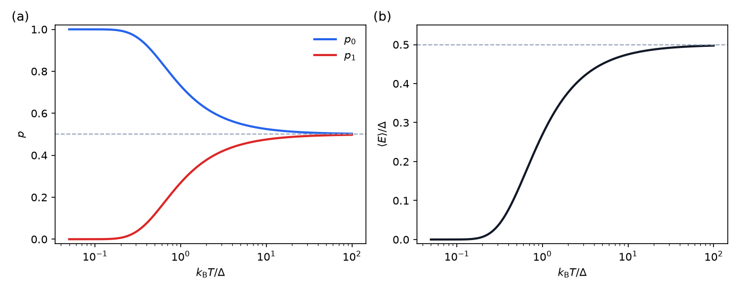
The two-level system against , on a logarithmic axis. (a) The ground-state occupation (blue) and the excited-state occupation (red); the dashed line is . (b) The mean energy in units of the gap, approaching (dashed) from below.
The limits are the point.
Cold, . , which vanishes: every system is in its ground state, and . Almost nothing happens until reaches about a fifth of the gap, which is why panel (a) is flat on its left.
Hot, . , so and both approach , and . The bath is so hot that one quantum more or less hardly changes its multiplicity, and the two states become equally likely.
Never inverted. For any positive temperature . Heating brings the populations toward equality, and no amount of heating passes it. What a population with more systems excited than not would mean is a question module 12 takes up.
Verify computationally
Every number below comes from thermolab.ensembles, which counts joint microstates exactly and
contains no random numbers. The energy quantum is throughout;
one quantum per bath oscillator puts the bath at , that is
.
1. The hand count. For the two-level system of step 2 on a bath of three oscillators with three quanta, listing the joint microstates one by one gives 16 of them: 10 with the system in its ground state and 6 with it excited, matching the binomial counts exactly.
2. Flat joint, curved marginal. With a bath of six oscillators and six quanta there are 714 joint microstates, each with probability exactly . The system is in its ground state in 462 of them and excited in 252: probabilities 0.647 and 0.353. On a bath of a thousand oscillators the excited probability is 0.33344, against the Boltzmann value . For this system the exact ratio is , which sits just above and approaches it as the bath grows.
3. The finite bath converges, at a rate you can quote.
4. The dropped term, measured. Step 5 predicted the correction to beyond . The exact count measures it directly, level by level, as
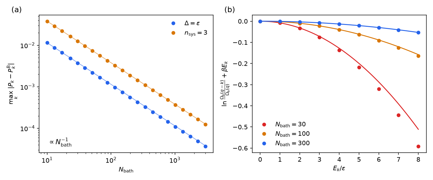
(a) The largest gap between the finite-bath marginal and the Boltzmann distribution, against bath size, for the two-level system with (blue) and the three-oscillator solid (orange); the lines have slope -1. (b) What the exact count adds to (dots), against the curvature term of step 5 (lines), for baths of 30 (red), 100 (orange) and 300 (blue) oscillators.
5. Reading off a bath. A student with only the counts can estimate the slope by adding and removing one quantum,
At one quantum per oscillator this differs from the exact slope by of itself at , at 40, at 160 and at 640 — a sixteenfold drop for every fourfold growth, second order. The exact slope itself differs from the infinite bath’s by at 10 oscillators and at 640: first order, the same as item 3.
6. The bath’s energy is not what sets the occupations. Put the same two-level system on three baths that each hold 100 quanta, but with 25, 100 and 400 oscillators. The excited occupation is 0.446, 0.334 and 0.167. The three baths have the same energy and very different slopes: their temperatures are 338, 106 and , and in each case the occupation matches the Boltzmann factor at that temperature to better than half a percent.
7. Two systems, one temperature. Put a two-level system with a gap of two quanta and a three-oscillator solid on the same bath of 5000 oscillators, and read each one’s own exponent off its own marginal. The two-level system gives , the solid 0.6931 to 0.6933 from its first three level ratios, and the bath’s own slope is 0.6930. Neither system has a temperature of its own.
Transfer the idea
The Boltzmann factor applies to any system in contact with any large bath, and “energy of the state” can be any energy at all. That generality is its power.
The barometric formula. A molecule in the atmosphere at height has gravitational energy . Treat the rest of the atmosphere as its bath, at temperature : the chance of finding it at height carries the factor , so the density, and with it the pressure, falls exponentially with height,
For nitrogen at the scale height is . The same result follows from hydrostatics plus the ideal-gas law; the counting argument and the macroscopic one agree, which is the point.
Arrhenius factors and defects. A reaction whose molecules must borrow an energy from their surroundings to get over a barrier proceeds at a rate carrying . A crystal site left empty costs a vacancy energy , so the fraction of empty sites is about — about 10-5 for at . Both are why chemistry and materials science are so sensitive to temperature.
Molecular and atomic excitation. The fraction of sodium atoms in a flame that are excited and can emit the yellow line is a Boltzmann factor with the degeneracies of the two levels in front, and it is small — under two in ten thousand. Astronomers read stellar temperatures from exactly such ratios.
Back to module 04. The Maxwell–Boltzmann distribution of molecular speeds that module 04 assumed is the Boltzmann factor applied to kinetic energy, . Module 12 derives it properly.
Back to module 10. “The reservoir” was an idealization there, “a body so large” that its temperature does not change. Step 5 says what large means, in numbers.
Looking ahead:
Module 12 takes from normalization constant to master key: , , and all follow from it, and is the free energy of module 10.
Module 13 repeats the counting of step 2 for a bath that trades particles as well as energy, and finds .
Module 15’s Monte Carlo simulation accepts a move with probability set by a ratio of Boltzmann factors — this module is its justification.
Module 17 replaces the levels of a single system with the levels of single particles, and the counting changes in an instructive way.
Worked examples
Try each one before opening its solution.
Worked example 1 — a bath of four. A two-level system with a gap of one quantum shares four quanta with a bath of three oscillators. Find the probability that it is excited, and compare with the value on a bath of three oscillators holding three quanta.
Solution
Ground: the bath holds four quanta in ways. Excited: three quanta in ways. So the excited probability is
With three quanta it was . The extra quantum warmed the bath, and a warmer bath excites the system more often. The exact ratio gives here and before.
Worked example 2 — a population ratio at room temperature. A molecule has an excited state above its ground state, both non-degenerate. What fraction of molecules is excited at ?
Solution
At , , so and
About two molecules in a hundred. A gap of is only four times , and that is already enough to empty the upper level almost completely.
Worked example 3 — the scale height. Estimate the scale height of an isothermal nitrogen atmosphere at , and the pressure at the summit of a mountain if it is at sea level.
Solution
A nitrogen molecule has mass , so
At , . The real atmosphere is colder aloft, which makes it thin a little faster; the international standard atmosphere, which builds that cooling in, gives . The isothermal assumption is the error, not the Boltzmann factor.
Worked example 4 — vacancies. Creating a vacancy in copper costs about . Estimate the fraction of empty lattice sites just below the melting point, , and at room temperature.
Solution
At , , so the fraction is , about one site in sixty thousand. At it is — which is why vacancies frozen in by quenching from a high temperature are far more numerous than room-temperature equilibrium allows.
Worked example 5 — how big a bath? You want the Boltzmann distribution to be accurate to in for system energies up to . How many oscillators must an Einstein bath in its equipartition regime have?
Solution
The dropped term is . At it is , and requiring it to be below 0.01 gives
A few hundred oscillators already make an excellent bath for a system that only ever holds a few . The bath does not need to be macroscopic; it needs to be large compared with the system’s energies.
Worked example 6 — sodium in a flame. The sodium D line comes from atoms in the level, above the ground level. The level holds six states and the level two. What fraction of sodium atoms is in the level in a flame at ?
Solution
At , , so
Fewer than two atoms in ten thousand are excited, and yet the flame glows bright yellow: there are a great many atoms. Leaving out the degeneracy factor would understate the population threefold.
Check your understanding
A small system has reached equilibrium with a large heat bath, and system plus bath together are isolated. Which microstates are equally probable?
A. Every joint microstate of system plus bath -- the system’s state together with the state of every bath oscillator. B. Every microstate of the small system, because it is in equilibrium. C. Every microstate of the bath, whatever the system is doing. D. None of them; equilibrium does not involve equal probabilities.
Check your answer
Correct answer: A — Every joint microstate of system plus bath -- the system’s state together with the state of every bath oscillator.
A. Right. The equal-probability postulate applies to an isolated system, and the isolated system here is the composite. The system’s own states are not equally probable: each is weighted by the number of bath microstates it leaves room for, which falls off exponentially with the energy the system takes.
B. This is the canonical-equal-probability misconception. Equal probability is a statement about an isolated system, and the small system is not isolated: it trades energy with the bath. Its microstates are weighted by exp(-E_s/(k_B T)). In the laboratory’s hand count, 16 joint microstates are each 1/16 likely, but the system is in its ground state in 10 of them and excited in only 6.
C. The bath is not isolated either: it trades energy with the system. What is fixed is the total, so it is the joint microstates -- system and bath together -- that are equally likely.
D. The whole derivation rests on equal probabilities, applied to the right thing: the joint microstates of the isolated composite. The Boltzmann factor is a consequence of that postulate, not a replacement for it.
Which pairing of ensemble, situation and probability rule is correct?
A. Canonical: a system exchanging energy with a bath at temperature T; P_s = exp(-E_s/(k_B T)) / Z. B. Canonical: a system exchanging energy with a bath; every microstate equally probable. C. Microcanonical: a system exchanging energy with a bath; P_s = exp(-E_s/(k_B T)) / Z. D. Microcanonical: an isolated system at fixed energy; P_s = exp(-E_s/(k_B T)) / Z.
Check your answer
Correct answer: A — Canonical: a system exchanging energy with a bath at temperature T; P_s = exp(-E_s/(k_B T)) / Z.
A. Right. The canonical ensemble is the small system’s view: its energy is not fixed, and its microstates are Boltzmann-weighted. The microcanonical ensemble is the isolated view: fixed energy, equal weights.
B. That pairs the canonical situation with the microcanonical rule. Equal weights belong to an isolated system at fixed energy. A system that trades energy with a bath has Boltzmann-weighted microstates.
C. The microcanonical ensemble describes an isolated system, whose energy is fixed; it exchanges nothing. The Boltzmann rule belongs to the canonical ensemble.
D. The situation is right but the rule is not. At fixed energy every accessible microstate has the same energy, and the postulate gives each the same probability, 1/Omega.
A two-level system in contact with a bath has a gap of Delta = 2 k_B T between its two non-degenerate states. What is the ratio of the excited population to the ground population, p_1 / p_0?
Check your answer
Correct answer: 0.1353 (± 0.002)
The Boltzmann factor gives p_1 / p_0 = exp(-Delta/(k_B T)) = exp(-2) = 0.135. If you answered 0.119, you computed the excited occupation p_1 = 1/(exp(2) + 1) rather than the ratio. If you answered 0.5, you gave both states equal weight, which holds only for an isolated system -- or at infinite temperature.
The Boltzmann distribution P_s = exp(-beta E_s) / Z was derived from P_s proportional to Omega_bath(U_tot - E_s). Which hypotheses does that step need?
A. The bath is much larger than the system’s energies, and the curvature of ln Omega_bath is negligible over them. B. Frequent collisions must shuffle the energy between system and bath. C. The system must be large, so that Stirling’s approximation applies to it. D. The system’s energy levels must be equally spaced.
Check your answer
Correct answer: A — The bath is much larger than the system’s energies, and the curvature of ln Omega_bath is negligible over them.
A. Right. Expanding ln Omega_bath about U_tot and stopping at the linear term needs both: E_s small compared with the bath’s energy, and E_s^2 times the second derivative of ln Omega_bath much less than one. The second derivative is -1/(k_B T^2 C_bath), so a big bath makes it vanish.
B. This is the misconception that the Boltzmann factor is a dynamical effect. The derivation counts joint microstates and uses no dynamics at all -- the laboratory’s enumeration contains no time and no collisions, and the exponential appears anyway. Collisions are one way a real system explores its microstates, not the origin of the exponential.
C. It is the bath that must be large, not the system. The Boltzmann distribution is exact enough for a single two-level system, provided its bath is big.
D. Nothing about the system’s levels enters the expansion, which is of the bath’s ln Omega. Any set of levels is Boltzmann-weighted; the laboratory uses both a two-level system and a solid with degenerate levels.
A two-level system sits on an Einstein bath at a fixed temperature. The largest gap between its exact occupations and the Boltzmann values is 1.4e-3 when the bath has 80 oscillators. The bath is doubled to 160 oscillators at the same temperature. By what factor is the gap divided?
Check your answer
Correct answer: 2.0 (± 0.1)
The term the Boltzmann derivation drops is E_s^2 / (2 k_B T^2 C_bath), and C_bath grows in proportion to the bath, so the gap falls as 1/N_bath: doubling the bath halves it, to about 7.0e-4. The laboratory measures an exponent of -1.004. If you answered sqrt(2), you carried over the N^(-1/2) of module 08’s fluctuations; that law is about a system’s spread, not about the error of treating a finite bath as infinite.
In P_s = exp(-beta E_s) / Z, what is beta?
A. The slope d(ln Omega)/dU of the bath’s multiplicity -- the bath’s 1/(k_B T), which the system inherits. B. 1/(k_B T) with T the temperature the small system has on its own. C. The system’s energy divided by k_B. D. A fitting constant chosen so that the probabilities add up to one.
Check your answer
Correct answer: A — The slope d(ln Omega)/dU of the bath’s multiplicity -- the bath’s 1/(k_B T), which the system inherits.
A. Right. beta came from expanding ln Omega_bath, so it is a property of the bath. The laboratory puts one two-level system on three baths holding the same energy but with 25, 100 and 400 oscillators: the excited occupation is 0.446, 0.334 and 0.167 -- each the Boltzmann value at that bath’s own temperature.
B. This is the misconception that temperature is a property of the system alone. Nothing of the small system entered beta: it is the slope of the bath’s ln Omega. Put the same system on baths of equal energy but different size and its occupations change, because the baths’ slopes differ.
C. beta is an inverse energy, 1/(k_B T), not an energy. And it does not belong to the system: it is the slope of the bath’s ln Omega.
D. That is the job of Z. beta has a meaning of its own: module 09’s 1/T = dS/dU, divided by k_B, evaluated on the bath.
In two or three sentences: every joint microstate of system plus bath is equally likely, yet the system’s own states are exponentially weighted. Explain how both can be true.
Check your answer
Equal probability applies to the joint microstates of the isolated composite, and the system’s probability of being in state s is the number of those joint microstates that have it there -- Omega_bath(U_tot - E_s) -- divided by the total. A system state with more energy leaves less for the bath, and the bath’s multiplicity falls steeply as its energy falls, so that state pairs with fewer joint microstates. A strong answer names the marginal (summing the flat joint distribution over the bath) and says why the fall is exponential: ln Omega of the bath drops by beta for each unit of energy removed.
The density of an isothermal atmosphere falls with height h as exp(-E/(k_B T)). Which energy E appears in the exponent?
A. The gravitational potential energy of one molecule, m g h. B. The kinetic energy of one molecule, (3/2) k_B T. C. The potential energy of the whole column of air above height h. D. The energy needed to ionize a molecule.
Check your answer
Correct answer: A — The gravitational potential energy of one molecule, m g h.
A. Right. The Boltzmann factor weights a molecule’s state by that state’s energy, and what changes with height is m g h. The scale height is k_B T/(m g), about 8.7 km for nitrogen at 288 K.
B. The kinetic energy is distributed the same way at every height in an isothermal atmosphere; it does not depend on h, so it cannot make the density fall with height.
C. The Boltzmann factor is about the state of one molecule in contact with a bath -- here the rest of the atmosphere. The column’s weight is what the macroscopic, hydrostatic derivation uses, and it gives the same answer.
D. Ionization energies are several electronvolts, far beyond k_B T in the lower atmosphere, and they do not change with height. The energy that changes with height is m g h.
A large number of two-level systems are in contact with a bath whose temperature is raised without limit. What does the fraction in the upper state approach?
A. One half, from below. B. One -- at high enough temperature every system is excited. C. Zero -- the excited state is always exponentially rare. D. It depends on the size of the gap Delta, even at infinite temperature.
Check your answer
Correct answer: A — One half, from below.
A. Right. p_1 = 1/(exp(Delta/(k_B T)) + 1), and as T grows exp(Delta/(k_B T)) approaches 1, so p_1 approaches 1/2. For any positive T the ratio p_1/p_0 = exp(-Delta/(k_B T)) is below one: heating equalizes the populations but never inverts them.
B. A hotter bath makes the upper state more likely, but never more likely than the lower one: the Boltzmann ratio exp(-Delta/(k_B T)) is below one at every positive temperature. An inverted population is not a very hot equilibrium state; module 12 says what it is.
C. The upper state is exponentially rare only when Delta is large compared with k_B T. At high temperature the exponent is small and the two states become nearly equally likely.
D. The gap sets how hot the bath must be before the populations approach each other, but not where they end up: as T grows without limit, p_1 approaches 1/2 for any gap.
A two-level system with a gap of one quantum shares 3 quanta with a bath of 3 Einstein oscillators; an Einstein solid of N oscillators holds q quanta in C(q + N - 1, q) ways. Counting joint microstates, what is the probability that the system is excited?
Check your answer
Correct answer: 0.375 (± 0.002)
Ground: the bath holds 3 quanta in C(5, 3) = 10 ways. Excited: it holds 2 in C(4, 2) = 6 ways. That is 16 joint microstates, each equally likely, so P(excited) = 6/16 = 0.375. If you answered 0.5, you weighted the system’s two states equally instead of counting what each leaves the bath.
Exam-style problems for this module — the ones worth doing with a pen — are collected in the problem set.
Explain it in your own words
Answer in a few sentences each.
A student writes: “In the canonical ensemble every microstate is equally probable.” Rewrite the sentence so that it is correct, and say precisely what was wrong with it.
Explain why temperature is a property of the bath that the system inherits, rather than a property the system brings. Use the three equal-energy baths of the verification.
The Boltzmann factor is often described as the result of molecules colliding and sharing energy. What does the counting argument deliver without any collisions, and what — if anything — are collisions still needed for?
Why does the derivation expand rather than itself? What would go wrong the other way?
Advanced: when the choice of ensemble stops mattering
The canonical ensemble lets the system’s energy fluctuate; the microcanonical ensemble fixes it exactly. For a small system the difference is enormous: a two-level system on a bath is sometimes excited and sometimes not. So why can module 04 be casual about which ensemble a real experiment realizes?
Because the canonical energy distribution of a large system is extraordinarily narrow. Consider an Einstein solid of oscillators on a bath. Each oscillator is independently Boltzmann-distributed, so the means and the variances of the oscillators add. With , one oscillator has mean energy and variance , so for the whole solid
with the mean number of quanta per oscillator. At one quantum per oscillator this is
: 1.41 for one oscillator, 0.14 for a hundred, 0.045 for a thousand, and
about for 1023. The library’s energy_moments computes these spreads
directly from the Boltzmann distribution over the solid’s levels, with no independence assumed,
and the test suite checks that it finds exactly this law.
At that point, fixing the energy exactly (microcanonical) or letting it fluctuate by a part in 1012 (canonical) changes nothing any instrument can detect, and every thermodynamic quantity computed either way agrees. This is the equivalence of ensembles in the thermodynamic limit. It is the same that narrowed module 08’s multiplicity peak and module 04’s pressure fluctuations, arriving by a third road.
The width is not a detail to be thrown away, though. Module 18 shows that for any system it is fixed by the heat capacity, — a fluctuation, measured at equilibrium, that tells you how the system responds when pushed. The Einstein result above is one instance of that relation.