Partition functions
The puzzle: the number you divide by
Module 11 introduced the partition function almost as an afterthought. A system in contact with a bath at temperature is found in microstate with probability , and is whatever makes those probabilities add up to one:
A bookkeeping constant, it seemed. Now do something that looks pointless with it: take its logarithm, and differentiate with respect to .
A harmonic oscillator of level spacing , against on a logarithmic axis. The four panels are, top to bottom, the mean energy , the entropy , the free energy (all three in units of or ) and the heat capacity in units of . The black curves are the exact results, computed from the probabilities level by level. The blue dots are computed from nothing but the single number at each temperature and its neighbours, by the difference formulas this module derives. The step between neighbours shrinks as the animation runs (its size relative to is printed in the top panel), and the dots settle onto the curves. The free energy needs no derivative, only itself, so its dots sit on the curve from the start.
Nothing in the dots knows the levels, the probabilities or the energy. Each dot comes from evaluated at three nearby temperatures, and yet the mean energy, the entropy, the free energy and the heat capacity all come out exactly.
The answer is a short calculation, and it makes the central object of equilibrium statistical mechanics. Once you have it, every thermodynamic quantity follows by differentiation; the rest of the course computes for one system after another.
Predict before you calculate
Commit to an answer for each of these before reading on. Write them down.
What does give — a quantity you already know, or something new? With what sign?
A salt of independent magnetic moments sits in a weak magnetic field. You halve the temperature at fixed field. Does its magnetization rise or fall, and by roughly what factor?
Keep adding energy to that salt until more moments point against the field than along it. Does its temperature rise without limit, jump to infinity, or turn negative? And if you then touch it to a body at room temperature, which way does heat flow?
A harmonic oscillator is very hot, . How much energy does it hold on average? And when it is very cold?
Explore the model
The laboratory has one machine at its centre: a function that is handed and nothing else, and returns , , and . It is run on three systems — a two-level system, a paramagnet of many independent moments, and a harmonic oscillator — and every output is checked against the system’s closed-form result. The laboratory then turns the paramagnet upside down, and last puts module 01’s simulated Einstein solid under the oscillator’s partition function.
The first animation follows the paramagnet’s entropy as energy is poured into it.
A paramagnet of moments. Left: its entropy against its energy in units of , from all moments along the field () to all against it (). The red segment is the tangent at the current energy (red dot). Right: the slope of that tangent, , in units of . It is positive on the left half, zero at the top of the dome, and negative on the right half, where adding energy removes microstates.
The second animation cools an oscillator.
A harmonic oscillator of level spacing , cooled from to . Left: the probability of each level (bars). Right: the heat capacity against (black curve); the dashed line is the equipartition value , and the red dot marks the current temperature. While several levels are occupied the heat capacity sits near the plateau; once only the ground level is left, it collapses.
Run the laboratory now, then come back. Four things are worth doing before you read on:
Hand the machine of a two-level system and compare its with module 11’s closed form.
Shrink the difference step by factors of two and watch the error; then keep shrinking it, and watch the error grow.
Halve the paramagnet’s temperature in a weak field, then in a strong one.
Put an inverted paramagnet in contact with a solid, make the solid as hot as you like, and find out which way the energy goes.
Derive the result
System and boundary. A system with a fixed list of energy levels — the level energies depend on nothing that changes during the argument — in contact with a large bath at temperature . Where the system has a volume, it is held fixed; where it sits in a field, the field is held fixed.
Independent variable. The temperature, through . Everything is a function of at fixed levels.
Sign convention. The course convention holds,
and with the levels fixed no work is done, : every change in the system’s mean energy is heat exchanged with the bath.
Route. Seven steps. The partition function is recalled; its first derivative gives , its second the energy fluctuations and ; the free energy follows and is checked against module 10; independent subsystems factorize; and two systems are worked in full — the paramagnet, which leads to negative temperatures, and the harmonic oscillator, which leads back to equipartition.
Step 1: the partition function, recalled
is a sum of Boltzmann factors, one per microstate. At low temperature only the lowest levels contribute; as rises more terms join in. So counts, roughly, how many microstates are thermally accessible — which already suggests it knows something.
Which levels matter. A level contributes to in proportion to . A level above the ground state is occupied less than one time in a hundred (); one up, less than once in twenty thousand. At any temperature only the levels within a few of the ground state matter, and the rest of the spectrum might as well not exist.
Step 2: the mean energy
Differentiate term by term. Each term’s derivative brings down its own energy:
Divide by , and the right-hand side becomes the average of over the Boltzmann distribution.
The logarithm is not decoration: , and dividing by is what turns the weighted sum into an average. That is the whole reason knows the energy. It is a sum of exponentials in , and differentiating an exponential brings its exponent down.
For module 11’s two-level system, and
module 11’s result, obtained this time without writing down a single probability.
Step 3: the heat capacity, and the fluctuations
Differentiate once more. is itself a ratio, so
The second derivative is the variance of the energy: in the canonical ensemble the system’s energy is not fixed, and this is how widely it spreads. The same second derivative is also , and converting from to with gives
With the levels fixed — fixed volume and particle number — every change of is heat, so is the heat capacity at constant volume, .
Two consequences follow at once. First, for every system in canonical equilibrium, because a variance cannot be negative: the thermal stability that module 09 demanded of is automatic here. Second, a quantity that describes the response of a system — how much heat it takes to warm it — is fixed by how much its energy fluctuates when left alone. Module 18 is built on that idea; here it costs three lines.
This is why rather than is the natural object. Its derivatives in are, up to sign, the cumulants of the energy distribution — the mean, the variance and the higher ones in turn. A function whose derivatives produce a distribution’s moments is called a generating function, and is the generating function of the canonical energy distribution. That is the answer to the puzzle: the normalization is not a single number but a function of , and its shape encodes every moment of the distribution it normalizes.
Step 4: the free energy — derived, not defined
The mean energy and its fluctuations came out of directly. The entropy and the free energy need one more step, and it is worth doing slowly, because it is where the statistical and the thermodynamic descriptions have to meet.
Module 10 defined the Helmholtz free energy , with no mention of microstates, and showed that . Consider the candidate
Take its temperature derivative. Using ,
So if we define , then , with the mean energy of step 2: the candidate has exactly the structure of module 10’s free energy. That is necessary, but it is not yet proof, because has so far only been named. What has to be shown is that is the thermodynamic entropy — the one module 07 defined through heat, and module 08 through counting. Two checks settle it.
It obeys Clausius. With the levels fixed, , so
since the first two terms cancel () and at fixed levels. Module 07’s entropy is defined, up to a constant, by exactly .
It counts microstates. Substituting into gives , so
the Gibbs entropy of the Boltzmann distribution. When all accessible microstates are equally probable, and this is module 08’s — which also fixes the constant that Clausius leaves free. As the system settles into its ground microstates and , their count.
That is a theorem, and it is worth being precise about why. Module 10’s was already defined — as a Legendre transform of , with nothing statistical about it. The statement says that a quantity computed from a list of energy levels equals that thermodynamic function, and it had to be checked: the entropy it implies had to obey Clausius and agree with the count of microstates. Writing as a definition would skip exactly the step that connects statistical mechanics to thermodynamics.
The payoff is enormous. Module 10 showed that is a fundamental relation: every equilibrium property at fixed temperature follows from it. So , computed from the levels, is the fundamental relation of the system — pressure, chemical potential and all, once the levels are allowed to depend on and .
Step 5: independent subsystems factorize
Most systems of interest are made of many parts. Suppose a system consists of subsystems that do not interact, so that a microstate of the whole is a list of one microstate for each part and its energy is the sum . The Boltzmann factor of a sum is a product, and the sum over all lists breaks into a product of sums.
Because is times , so is everything derived from it: , , , and the variance are all extensive. The spread, though, grows only as the square root:
the same that narrowed module 08’s multiplicity peak and module 11’s canonical energy distribution, now arriving from a derivative of .
“Distinguishable” matters. A crystal’s magnetic moments sit on labelled lattice sites, and swapping two of them gives a different microstate. Identical gas molecules are not labelled, and counting every permutation as a new microstate overcounts by . That correction is the subject of the advanced section; nothing in the core needs it.
Step 6: the paramagnet, worked in full
A paramagnet is a material whose atoms carry permanent magnetic moments that do not interact with one another. In a field , a moment pointing along the field has energy and one pointing against it (a spin-1/2 moment, like an unpaired electron, has only these two orientations). One moment is a two-level system with gap , and with ,
The energy follows from step 2, and the net moment along the field — the magnetization — from :
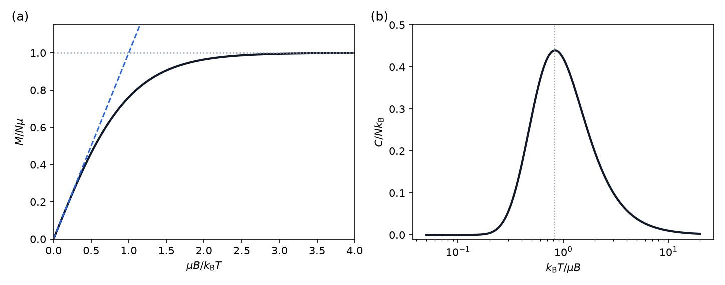
(a) The paramagnet’s magnetization, , against (black), with the Curie law (dashed) and saturation at (dotted). (b) Its heat capacity per moment, , against on a logarithmic axis: a single peak — the Schottky anomaly — near , dying at both ends.
The two limits are the physics.
Weak field or high temperature, . , so
This is Curie’s law: the magnetization is proportional to . Halve the temperature and it doubles. The field tries to align the moments, the bath tries to scramble them, and the outcome depends only on the ratio of the two.
Strong field or low temperature, . , so : every moment is aligned, and no further field can add to it. This is saturation.
The heat capacity, from step 3, is a two-level system’s for each moment, . It vanishes when cold (every moment aligned, nothing to excite) and when hot (the moments already split half and half, and further heating changes nothing), with a peak in between. Such a peak in the measured heat capacity of a solid is the fingerprint of a set of two-level systems hidden in it.
The paramagnet at fixed energy. So far the paramagnet has been in contact with a bath. Now isolate it and count instead, as module 08 did for coins. With of the moments pointing against the field, the energy is
running from (all aligned) to (all reversed), and the number of microstates is the binomial coefficient . The entropy is the dome of the second animation: zero at both ends, where there is only one way to arrange the moments, and largest at , where half point each way.
Now apply module 09’s definition of temperature, . A moment reversed costs , and by Stirling , so
For — more moments along the field than against — is positive, and inverting gives , the Boltzmann ratio of the canonical calculation. At the dome is flat: , an infinite temperature. And for the dome slopes down: adding energy removes microstates, is negative, and so is .
What does a negative temperature mean? Not what the number suggests. The honest way to find out is to ask what temperature is for: deciding which way heat flows.
Put the paramagnet (body 1) in contact with any other body (body 2), the pair isolated. Energy passes into body 1 and leaves body 2, and the total entropy changes by
The second law, in module 08’s counting form, says the pair moves toward more microstates, . So energy flows into body 1 when and out of it when : heat flows from the body with the smaller to the body with the larger one. For two positive temperatures this is the familiar rule, hot to cold. But now take an inverted paramagnet, , and any ordinary body at any positive temperature, .
A negative temperature is not below absolute zero. It is above infinite temperature. The paramagnet with more moments reversed than aligned holds more energy than it would at any positive temperature — at the moments split exactly half and half — and it will give some of that energy to anything at a positive temperature it touches, however hot. The quantity that orders hotness is , not ; merely has an awkward jump from to in the middle, at the top of the dome, where nothing physical happens at all.
This is also why module 11 found that heating never inverts a two-level population: a bath at positive temperature has and can only bring the system to . An inverted population is not a very hot equilibrium with a positive-temperature bath; it has to be made some other way, and the advanced section says how.
Step 7: the harmonic oscillator, and equipartition recovered
The last system has infinitely many levels, equally spaced: for — a quantum harmonic oscillator, and one of module 01’s Einstein-solid oscillators, with its energy quantum. With the partition function is a geometric series,
and step 2 gives
The is the zero-point energy, the ground level’s own energy. It shifts and by a constant and changes neither nor ; module 01, counting quanta above the ground state, simply left it out. Step 3 gives the heat capacity,
Hot, . Expanding the exponential, , and . This is equipartition. Module 06 counted for every quadratic term in the energy; an oscillator has two, its kinetic and its potential energy, and holds . The rule modules 04 and 06 used by assumption is here a limit of a partition function.
Cold, . The first excited level is out of reach, the oscillator sits in its ground state, and
exponentially small. The oscillator can no longer absorb heat in small amounts: its smallest bite is a whole quantum , which the bath almost never supplies. The degree of freedom has frozen out.
A solid of atoms has vibrational modes. If each held , its heat capacity would be at every temperature — the Dulong–Petit law, which fits many solids at room temperature and fails for all of them when cold, because the modes freeze out. How they freeze out, mode by mode, is module 16.
Verify computationally
Every number below comes from thermolab.partition. Level spacings are
for the two-level gap and the oscillator quantum
(), and the paramagnet’s moments are Bohr magnetons,
, in
().
1. The machine. thermo_from_z is handed a function returning , and nothing else.
It differentiates in with central differences,
then sets , and . The step is a fixed fraction of itself.
2. The step, and why it cannot be too small. Both difference formulas are second order: their truncation error falls as . Measured on the oscillator at , halving the step from to divides the error of by 4.02, 4.00, 4.00, 4.00.
The rise is roundoff error. The formulas subtract values of that agree in more and more of their sixteen significant digits as shrinks, and the difference is left with fewer and fewer correct ones. The first difference divides that loss by , the second by , which is why suffers first. The best step balances the two errors: about for and for , with the float’s relative precision, and those are the defaults. The same cancellation is what degrades in item 1’s tails. Where is exponentially small, barely curves, and its curvature is buried under the digits it shares at three neighbouring points. There a sum over the levels, which never subtracts, is the better tool.
3. , tested against module 10’s . The laboratory computes the oscillator’s free energy twice. Once from . Once as , with and the Gibbs entropy both summed from the probabilities, so that no appears in the second computation at all. At 20, 72.4 and the two agree to , and exactly — rounding in the last digit. The entropy that implies is the entropy the probabilities carry, which is step 4’s second check made numerical.
4. The paramagnet’s magnetization. For 104 electron moments in :
| (K) | 300 | 150 | 10 | 1 | 0.3 | 0.1 |
|---|---|---|---|---|---|---|
| 0.00224 | 0.00448 | 0.0671 | 0.586 | 0.978 | 1.000 | |
| Curie law | 0.00224 | 0.00448 | 0.0672 | 0.672 | 2.24 | 6.72 |
Halving the temperature from 300 to multiplies by 1.99999. Below about the Curie law predicts more than every moment can give, and the true curve saturates.
5. Fluctuations shrink as . From the reconstructed second derivative of at , the relative energy fluctuation of the paramagnet is 0.437 for 10 moments, 0.0437 for 1000 and 0.00138 for 106. The fitted exponent is -0.5000000, and going from 104 to 106 moments divides the fluctuation by 10.0000.
6. The dome, and the heat that leaves it. For moments the entropy rises from 0 to at (against the of Stirling’s leading term), and the slope read off by central difference gives
| moments reversed | 10 | 30 | 49 | 50 | 51 | 70 | 85 |
|---|---|---|---|---|---|---|---|
| (K) | 0.62 | 1.60 | 33.9 | -33.9 | -1.60 | -0.79 |
— symmetric about the peak, with the sign flipping as the tangent passes over the top.
Even the solid, whose own temperature is more than a thousand times the magnitude of the paramagnet’s, takes energy from it. The count settles the paramagnet at 50 reversed moments — as close to as a finite system gets — never at a positive temperature below the solid’s, which would mean giving up still more.
7. Equipartition, and freeze-out. The oscillator’s mean energy per , measured above the ground state, is 0.9950 at , 0.951 at , 0.582 at and 0.0005 at . Its heat capacity is , , and at 10, 1, 0.2 and .
8. Module 01’s solid, under the oscillator’s partition function. Module 01 simulated two Einstein solids trading quanta and read each one’s temperature by equipartition, per oscillator. Its model specification warned that this reading fails when cold. The oscillator partition function supplies the exact reading: inverting above the ground state,
which is also module 09’s temperature, from the slope of the Einstein solid’s — the two agree to 10-14. For it is equipartition’s reading plus half a quantum.
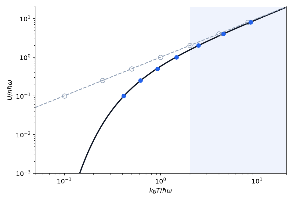
Mean quanta per oscillator against . Black: the oscillator partition function’s above the ground state. Dashed: equipartition, , module 01’s reading. Blue: the endpoints of module 01’s simulation at seven energies — two solids of 40 oscillators, 8 seeds each — placed at the temperature the partition function assigns them. Grey circles: the same endpoints at the temperature module 01’s equipartition reading assigns. The shaded band, , is where the two readings differ by less than about a quarter.
The simulation supplies the energies; the partition function supplies the thermometer. The simulation cannot choose between the two thermometers: both say that two solids of one quantum size settle at equal energy per oscillator, and that is all it shows. What decides between them is module 09’s slope of , which the partition function reproduces and equipartition only approaches. The overlay illustrates, and the derivation of step 7 establishes: nothing in these numbers proves the oscillator formula, which rests on the levels being .
Transfer the idea
The recipe — list the levels, sum the Boltzmann factors, differentiate the logarithm — works for any system whose levels you know.
Frozen molecular vibrations. A nitrogen molecule vibrates with a quantum of . At its vibrational heat capacity is — frozen out — which is why module 06 could treat air as a diatomic gas with , counting rotations and not vibrations. At the vibration contributes and at : the heat capacity of hot air climbs as the mode thaws.
The Schottky anomaly. Any solid containing a set of two-level systems — impurity moments, tunnelling defects — shows a bump in its heat capacity near , peaking at per two-level system. Measuring the bump’s position reads off the hidden gap.
Defect concentrations. A lattice site that is either filled (energy 0) or vacant (energy ) is a two-level system, and the vacant fraction is — module 11’s Arrhenius factor, corrected for the denominator. For at the correction is one part in 105.
Chemical equilibrium. A molecule that can exist as isomer A or isomer B, the latter higher, is one system with two groups of levels, and the ratio of the two populations is the ratio of the two groups’ partition functions — with non-degenerate ground levels, . Module 13 generalizes this to reactions that change the number of molecules.
Magnetic refrigeration. Magnetize a paramagnet at low temperature, let the heat of magnetization flow away, isolate it and switch the field off: its entropy cannot change, but the entropy of a paramagnet depends only on , so falls in proportion to . This is how laboratories reach millikelvin temperatures, and every step of it is a statement about .
Looking ahead:
Module 13 lets the bath exchange particles as well as energy, and the Boltzmann factor gains a term for the particles each state holds, .
Module 15 meets moments that interact: no longer factorizes, and the paramagnet becomes a magnet.
Module 16 sums oscillator partition functions over every mode of a solid (Einstein and Debye) and of the electromagnetic field (Planck).
Module 17 trades single-system levels for single-particle levels.
Module 18 takes from here and uses it.
Worked examples
Try each one before opening its solution.
Worked example 1 — everything from one sum. A two-level system has gap . Find , , , and .
Worked example 2 — aligning electron moments. Electron moments in a field. What fraction of the saturation magnetization is reached at ? How cold must the salt be for ?
Solution
At , , and : about two moments in a thousand, net. For , gives , so
A field of is a weak perturbation at room temperature; aligning electron moments takes a fraction of a kelvin.
Worked example 3 — why air has five, not seven. Nitrogen’s vibration has . Estimate its contribution to per molecule at and .
Solution
With , . At , and . At , and . Equipartition would give the full — the two quadratic terms that would lift a diatomic gas from to per molecule. At room temperature they are frozen out.
Worked example 4 — which way does the heat go? A crystal’s nuclear moments are prepared with of them reversed; its temperature is . It is touched to a copper block at . Which way does heat flow, and does the answer change if the copper is at ?
Solution
The moments have ; the copper has at either temperature. Heat flows from smaller to larger, so it flows from the moments to the copper in both cases. The negative-temperature system is hotter than the copper at any positive temperature. The reversed moments relax back toward alignment and the copper warms.
Worked example 5 — a zero-point question. An oscillator of quantum is at . What is its mean energy with the zero point, and without it? Which of , , and depend on the choice?
Solution
with the zero point, without. Removing the zero point multiplies every Boltzmann factor by , so gains : and both drop by , and and are unchanged. Only differences of energy are physical here.
Worked example 6 — how steady is a macroscopic magnet? The laboratory finds for the paramagnet at in . What is it for a sample of 1020 moments?
Solution
. The energy of a macroscopic sample in canonical equilibrium is sharp to about a part in ten billion, even though each moment’s own energy swings between and .
Check your understanding
A system with fixed energy levels is in contact with a bath. What is -d(ln Z)/d(beta), with beta = 1/(k_B T)?
A. The mean energy U of the system. B. The free energy F of the system. C. Nothing physical -- Z only normalizes the probabilities, so its derivative has no meaning. D. The entropy S of the system, divided by k_B.
Check your answer
Correct answer: A — The mean energy U of the system.
A. Right. Differentiating Z = sum_s exp(-beta E_s) brings down -E_s in every term, and dividing by Z -- which is what the logarithm does -- turns that sum into an average: -d(ln Z)/d(beta) = sum_s E_s P_s = U. The second derivative gives the variance of the energy.
B. The free energy is -k_B T ln Z itself, with no derivative taken. Differentiating ln Z in beta gives the mean energy; U and F differ by TS.
C. Z is a function of beta, not a single number, and its shape carries the energy distribution. Its logarithm’s first derivative is -U and its second is the variance of E: ln Z is the generating function of the canonical energy distribution.
D. The entropy needs both ln Z and its derivative: S = k_B (ln Z + beta U). The derivative alone is -U.
A two-level system has levels 0 and Delta, with Delta = 2 k_B T. Using U = -d(ln Z)/d(beta), what is its mean energy, as a multiple of Delta?
Check your answer
Correct answer: 0.1192 (± 0.002)
ln Z = ln(1 + exp(-beta Delta)), so U = Delta exp(-beta Delta)/(1 + exp(-beta Delta)) = Delta/(exp(2) + 1) = 0.119 Delta. If you answered 0.135, you gave the population ratio exp(-2), not the excited fraction. If you answered 0.5, you gave the infinite-temperature limit.
What is the status of the statement F = -k_B T ln Z?
A. A theorem -- it holds because the entropy it implies was checked to obey dS = dQ/T and to equal the Gibbs count of microstates, so it is module 10’s F = U - TS. B. A definition -- statistical mechanics defines the free energy as -k_B T ln Z. C. An approximation, valid only for large systems. D. An empirical law, found by measuring free energies.
Check your answer
Correct answer: A — A theorem -- it holds because the entropy it implies was checked to obey dS = dQ/T and to equal the Gibbs count of microstates, so it is module 10’s F = U - TS.
A. Right. Module 10 defined F = U - TS before any ensemble existed. That -k_B T ln Z equals it had to be shown: its entropy k_B (ln Z + beta U) obeys Clausius’s dS = dQ/T at fixed levels and equals -k_B sum P ln P. The laboratory computes -k_B T ln Z and U - TS independently and finds them equal to rounding.
B. This is the misconception that F = -k_B T ln Z is a definition. The free energy was already defined, thermodynamically, as U - TS. Calling the formula a definition skips the step that connects the two descriptions: checking that the entropy it implies is the thermodynamic entropy.
C. Nothing in the derivation needs a large system: it holds exactly for any system with fixed levels in contact with a bath, even a single two-level system.
D. It is derived, not measured: from the Boltzmann distribution plus two checks on the entropy. Experiments test the model levels, not the formula.
A crystal’s magnetic moments have been prepared with more of them pointing against the field than along it, so their temperature is negative. The crystal is touched to a copper block at room temperature. Which way does heat flow?
A. Out of the moments and into the copper -- a negative-temperature system is hotter than any positive-temperature one. B. Into the moments -- a negative temperature is colder than absolute zero, so they are colder than the copper. C. No heat flows, because the two temperatures cannot be compared. D. It depends on whether the copper is hotter than the magnitude of the negative temperature.
Check your answer
Correct answer: A — Out of the moments and into the copper -- a negative-temperature system is hotter than any positive-temperature one.
A. Right. The total entropy changes by k_B (beta_1 - beta_2) dU_1, and it must rise. With beta_1 < 0 < beta_2, that needs dU_1 < 0. In the laboratory an inverted paramagnet gives energy to a solid at 0.56 K, 14 K and 1344 K alike. Ordered by hotness, negative temperatures lie above T = infinity.
B. This is the misconception that negative temperature means colder than absolute zero. The moments hold more energy than at any positive temperature -- at T = infinity they split half and half, and here more point against the field. They give energy to anything at a positive temperature, however hot.
C. They can be compared through beta = (1/k_B) dS/dU, which runs continuously from positive through zero to negative. Heat flows from the smaller beta to the larger.
D. The magnitude does not matter. Every negative beta is smaller than every positive beta, so energy leaves the moments whatever the copper’s temperature -- the laboratory’s 1344 K solid still takes energy from a -0.79 K paramagnet.
A paramagnet is in a weak field, mu B << k_B T. Its temperature is halved at fixed field. By what factor does its magnetization change?
Check your answer
Correct answer: 2.0 (± 0.05)
In the Curie regime M = N mu^2 B/(k_B T), so halving T doubles M. The laboratory finds a factor of 1.99999 between 300 K and 150 K in a 1 T field. If you answered 1, you were thinking of saturation, where every moment is already aligned. If you answered 4, you squared the temperature: the Curie law is 1/T, not 1/T^2.
A harmonic oscillator with level spacing hbaromega is in contact with a bath at k_B T = hbaromega/20. What is its heat capacity?
A. Exponentially small, about k_B (hbaromega/(k_B T))^2 exp(-hbaromega/(k_B T)) -- the oscillator has frozen out. B. k_B, as for every oscillator at every temperature -- which is why a solid has C = 3 N k_B. C. k_B / 2, because only the kinetic energy still counts. D. Infinite, because the energy changes abruptly between levels.
Check your answer
Correct answer: A — Exponentially small, about k_B (hbaromega/(k_B T))^2 exp(-hbaromega/(k_B T)) -- the oscillator has frozen out.
A. Right. At k_B T << hbar*omega the first excited level is out of reach, and the smallest amount of energy the oscillator can take is a whole quantum the bath almost never supplies. Here C = 400 exp(-20) k_B, about 8e-7 k_B.
B. This is the misconception that the Dulong-Petit value holds at all temperatures. C = k_B per oscillator is equipartition, the high-temperature limit k_B T >> hbar*omega. When cold the oscillator freezes out, and solids’ heat capacities fall toward zero -- module 16 follows this for real solids.
C. Freezing out is not a matter of losing one quadratic term: the whole oscillator stops absorbing heat, because its excited levels are out of reach. C falls exponentially, not by half.
D. The canonical mean energy is a smooth function of temperature, so C is finite; and when cold it is tiny, since almost no oscillator is excited at all.
Two paramagnets are at the same temperature and in the same field: one has N = 10^4 moments, the other N = 10^6. By what factor is the relative energy fluctuation sigma_E/|U| of the small one larger than that of the large one?
Check your answer
Correct answer: 10.0 (± 0.2)
For independent moments ln Z_N = N ln z, so U grows as N and the variance d^2(ln Z)/d(beta)^2 also grows as N; sigma_E grows as sqrt(N) and sigma_E/|U| falls as N^(-1/2). A hundredfold increase in N divides it by 10. If you answered 100, you let sigma_E stay fixed while U grew; if you answered 1, you treated the relative spread as a property of the material rather than of the sample’s size.
U is reconstructed from ln Z with the central difference -[ln Z(beta + h) - ln Z(beta - h)]/(2h). The step h is halved, and it is still far larger than the step at which roundoff matters. What happens to the error?
A. It falls by a factor of about four, because the central difference is second order. B. It halves, because the error is proportional to the step. C. It does not change, because the formula is exact for any step. D. It grows, because a smaller step always makes the subtraction less accurate.
Check your answer
Correct answer: A — It falls by a factor of about four, because the central difference is second order.
A. Right. The truncation error of a central difference is proportional to h^2. The laboratory measures an order of 2.002 +/- 0.001: each halving divides the error by 4.00.
B. That is a one-sided difference, first order. The symmetric formula cancels the h term, and the leading error is h^2 f’‘’/6.
C. It is exact only when ln Z is a quadratic in beta, which it never is here. The error is proportional to h^2 and to the third derivative of ln Z.
D. That is roundoff, and it wins only for very small steps -- in the laboratory below about 1e-5 of beta for U. Above that, truncation dominates and a smaller step is better.
In three or four sentences: why does the normalization constant Z determine a system’s thermodynamics, and what had to be checked before writing F = -k_B T ln Z?
Check your answer
Z is a function of beta, and each term exp(-beta E_s) carries its state’s energy in the exponent, so differentiating ln Z in beta produces averages over the Boltzmann distribution: the first derivative is -U, the second the variance of E, which equals k_B T^2 C_V. ln Z is thus the generating function of the energy distribution. For F: the free energy had already been defined in module 10 as U - TS, so -k_B T ln Z had to be shown to equal it -- the entropy it implies, k_B (ln Z + beta U), was checked to obey dS = dQ/T at fixed levels and to equal the Gibbs sum -k_B sum P ln P. A strong answer names both checks and calls the result a theorem.
Exam-style problems for this module — the ones worth doing with a pen — are collected in the problem set.
Explain it in your own words
Answer in a few sentences each.
A classmate says: “ is just the normalization constant; the physics is in the Boltzmann factors.” Convince them otherwise, using step 2.
Rewrite this sentence so that it is correct: “Negative temperature means colder than absolute zero.” Say what has to do with it.
Is a definition or a theorem? What had to be checked before it could be written down?
Why does a harmonic oscillator stop absorbing heat when it is cold, while a classical oscillator — module 06’s — never does?
Advanced: the ideal gas, the Gibbs factor, and real negative temperatures
One particle in a box. A particle of mass in a box of volume has translational levels too closely spaced to see individually at ordinary temperatures. Counting them — one state per cell of volume in position–momentum space, a result stated here and derived in module 17 — turns the sum into an integral with the value
where is the thermal wavelength: for argon at . So is, roughly, the number of thermal-wavelength cubes that fit in the box. Step 2 gives at once, since — equipartition for three quadratic terms.
N particles, and the factor N! If the particles were distinguishable, step 5 would give . But identical particles are not labelled: exchanging two of them does not produce a new microstate, and counts each configuration times. The corrected partition function is
The correction is not cosmetic. Without it the entropy is not extensive: doubling and together should double , but with it overshoots by — the entropy of mixing two samples of the same gas, which is module 08’s Gibbs paradox. With the and Stirling’s , step 4 gives
the Sackur–Tetrode equation that module 09 stated. For argon at and
, and . The test suite checks
that thermo_from_z applied to this reproduces module 09’s formula, and that dropping
the breaks extensivity by exactly .
The derivation also says when it fails. means the particles are far apart compared with their thermal wavelength, so that no two ever compete for one state and dividing by is enough. When approaches — dense, cold gases, electrons in a metal — it is not, and module 17’s quantum statistics take over.
Negative temperatures in the laboratory. A population with more moments against the field than along it cannot be reached by heating, but it can be reached by reversing the field faster than the moments can follow. Purcell and Pound did exactly this in 1951 with the nuclear moments of lithium in a LiF crystal: after a sudden reversal of the field, the nuclear spins were at a negative temperature and relaxed back through over minutes, the timescale on which they exchanged energy with the lattice. Every laser relies on a population inversion in the same sense: its working levels are held at a negative temperature, and the light it emits is the energy that flows out of them.
Two caveats keep this honest. The spins can be assigned a temperature only because they reach equilibrium among themselves much faster than they reach it with the lattice; the spin system is then isolated enough to have its own . And negative temperatures exist only for degrees of freedom with an energy ceiling. The same crystal’s vibrations have none, so the crystal as a whole is never at a negative temperature.