Fluctuations and transport — the noise that carries heat
Fluctuations and transport
The puzzle: the noise we kept throwing away
For seventeen modules the course has treated fluctuations as noise around the signal. Module 03’s walkers scattered about their average, module 04’s pressure gauge jittered, and the energy of module 11’s small system on a bath wandered up and down. Each time the lesson was the same: the relative scatter falls as , so for anything macroscopic it can be averaged away and forgotten.
Now put a drop of ink into a glass of perfectly still water, or warm one end of a metal rod, or stir honey and watch it drag. Ink spreads with no current to carry it. Heat crosses the rod with nothing flowing. The honey resists being sheared. Nothing pushes in any of these: there is no pressure difference behind the ink and no wind across the rod. The only thing moving is the molecules, at random, in exactly the motion the course has been averaging away.
And the numbers are strange. A dye molecule in water moves at over a hundred metres per second, yet a dye cloud takes about a day to spread over a centimetre, and would need decades to cross a metre. Module 12 adds a stranger fact still: for a system on a heat bath, the size of its energy noise is fixed by its heat capacity, . The noise is a property of the material.
The answer adds one idea to the course: memory. How far a cloud of molecules spreads, how hard a gas resists shearing and how well it conducts heat are all fixed by how long a molecule remembers its velocity before a collision makes it forget.
Predict before you calculate
Commit to an answer for each of these before reading on. Write them down.
A simulation of two-level systems on a heat bath shows the total energy fluctuating. You double . Does the relative fluctuation halve, fall by a factor of , or stay the same?
A layer of dye at the bottom of a tall jar of set gelatin, where nothing can flow, has after one day coloured the gelatin up to above the layer. How high will the colour reach after four days?
You pump half of the gas out of a sealed container at fixed temperature. Does the viscosity of the gas that remains halve, stay the same, or double?
You run the same simulation of a system on a bath ten times longer. Does the fluctuation of its energy get smaller?
Explore the model
The laboratory has four explorers. The first releases a cloud of up to ten thousand random walkers at the origin and shows its histogram at a time you choose, with the diffusion equation’s prediction drawn over it, and its mean squared displacement on linear or logarithmic axes; a switch gives the walkers a memory of their last step. The second measures the relative energy fluctuation of two-level systems for from 16 to 4096. The third estimates the mean free path, collision rate, viscosity and thermal conductivity of helium, nitrogen or argon at the temperature and pressure you choose, against measured values. The fourth races a diffusion front against a front moving at a steady speed. Then the laboratory runs the experiments this module is built on: a heat capacity read off the noise, the law, the diffusion coefficient measured three ways for walkers with and without memory, module 04’s gas failing to diffuse, the transport coefficients of real gases, and Avogadro’s number from Brownian motion.
Ten thousand independent walkers, each stepping one step length left or right every time , all released at the origin, as time runs from to . Left: the histogram of their positions, one bar per reachable site, with the diffusion equation’s point-source solution for drawn over it in blue — computed from and , not fitted to the bars. The cloud spreads and flattens and its area stays one. Right: the mean squared displacement on logarithmic axes, growing along the slope-one line (dashed). Its fitted slope from 100 to 1000 steps is 1.005.
Run the laboratory now, then come back. Four things are worth doing before you read on:
In the cloud explorer, compare the histogram at 250 steps with the one at 1000. How much wider is it? How much lower is its peak?
Switch the logarithmic axes on for the mean squared displacement, then give the walkers a strong memory. What happens to the slope at early times?
In the fluctuation explorer, multiply by four. By what factor does the relative fluctuation fall?
In the transport calculator, lower the pressure of nitrogen from 105 to and watch the mean free path and the viscosity.
Derive the result
System and boundary. Two kinds of system. For the fluctuations: a body of fixed volume and particle number in contact with a heat bath at temperature , so that its energy is free to fluctuate (module 11’s canonical ensemble). For transport: a dilute gas, or a suspension of small particles in a liquid, in which one species is tagged and followed; the tagged particles do not interact with one another.
Independent variables. The temperature , the number density , the molecular mass and size ; for the random walk, the step length , the step time and the persistence .
Sign convention. The course convention, , holds. It is exercised in step 8: heat conducted into a rigid slab does no work, , so every joule that crosses its face down the temperature gradient becomes internal energy, .
Units. SI throughout, with explicit. Walkers live on a line, so their is one-dimensional, . A real gas is three-dimensional, where — three one-dimensional walks, one per axis, with the same . The dimension is stated beside every formula that depends on it.
Route. Nine steps. Read module 12’s fluctuation identity as an instrument, and see why it makes big systems steady. Take module 03’s random walk to its continuum limit, which is the diffusion equation, and solve it. Give the walker a memory of its velocity, which brings in the Green–Kubo relation and explains both the ballistic start and the slowness of diffusion. Balance drift against diffusion to get the Einstein relation, which turned Brownian motion into a measurement of Avogadro’s number. Then count collisions in a gas — the mean free path that module 04’s model left out — and use one random flight to estimate all three transport coefficients, before naming the assumption all of them share.
Step 1: the noise is a heat capacity
Module 12 derived it in three lines. The canonical mean energy is , the second derivative of is the variance of the energy, and converting from to gives
Module 12 drew one consequence: , because a variance cannot be negative. This module draws another. The identity is an instrument. Record the energy of a system on a bath — in a simulation, or for a nanoscale object, in a laboratory — and its heat capacity follows from the scatter, at one temperature, with nothing heated:
Take module 04’s ideal gas, drawn canonically. Each of its quadratic degrees of freedom per particle — three for a monatomic gas — carries an energy whose variance is , and for independent degrees of freedom variances add. So , and the instrument reads : equipartition, measured from noise.
Two warnings come with the instrument. First, the identity is canonical. A system whose energy is fixed — microcanonical, like module 04’s gas drawn with its energy rescaled to an exact value — has no energy fluctuation at all, and the instrument would read , which is wrong. The bath is part of the measurement. Second, the fluctuation is not an error. A longer record measures more precisely; it does not make it smaller, because it is not a property of the record. It is .
Step 2: why large systems look steady
and are extensive: for independent subsystems, or for any large system made of weakly coupled parts, both grow in proportion to . Then
For two-level systems at , where a fraction of them is excited, the ratio is : 0.41 for 16 systems, 0.026 for 4096, and for a mole. Module 11’s advanced section found the same law for an Einstein solid by a direct calculation; here it follows for any system from the identity alone. At a part in 1012 no instrument can tell whether the energy is fixed (microcanonical) or merely almost fixed (canonical), and the two ensembles give the same thermodynamics. That is the equivalence of ensembles, and the reason the course could use whichever was convenient.
The identity holds only for the ensemble whose energy fluctuates; the agreement between ensembles holds only for large . They are compatible because the fluctuation the identity measures, although it equals a material property, is too small to matter for anything else.
Step 3: from random walk to the diffusion equation
Module 03’s walker steps a distance to the left or to the right, with equal probability, every time . Let be the probability of finding it at at time . To be at at time it must have been one step to either side at time , and taken the step that brought it here:
This is a master equation: a bookkeeping rule for probability, nothing more. Now look at it on scales much longer than and times much longer than , where changes smoothly, and expand both sides by Taylor’s theorem:
The first-derivative terms in cancel between the two sides of the walker — that is where “unbiased” enters. Divide by and let and shrink together with held fixed. The omitted terms, of order and , vanish in that limit, and what remains is
The same equation holds for the number density of many independent walkers. Look at it from the point of view of a single plane between two sites. In one step, half the walkers just to its left cross it to the right, and half of those just to its right cross to the left. The net flow per unit time is half the difference, which on a smooth profile is
That is Fick’s law, and it explains the flux down a concentration gradient without any force. Nothing pushes the walkers away from the crowded side; there are simply more of them there to step across. (This is the flux of independent particles. For interacting ones, module 13 showed that the gradient that drives the flow is the chemical potential’s, not the concentration’s.) Combined with the conservation of walkers, , Fick’s law gives the diffusion equation again.
Both hypotheses matter. If a step depends on the one before, as in module 03’s persistent walk, the probability of being at at time depends on which way the walker was moving, and the master equation needs a second variable; step 5 shows what the memory does to . If a step has no finite variance, as for module 03’s Cauchy walker, the Taylor expansion has no second-order term to keep, and there is no diffusion equation at all.
Step 4: the spreading cloud, and why diffusion is slow
Release a cloud of walkers at the origin at . The solution of the diffusion equation that starts as a point is the Green’s function
a Gaussian of variance — module 03’s central limit theorem, now with physical units. (Check it by differentiating: and both equal .) Its mean squared displacement is
A front, defined as the place where the concentration has reached a given fraction of its source, moves the same way. A layer of dye filling at , with clear water above it, spreads as
which depends on and only through . The quarter-strength contour sits at : four times as long, twice as far.
That is why diffusion is fast over short distances and hopelessly slow over long ones. The time to spread over a distance grows as . A small molecule in water has : it spreads across a cell in about , across a centimetre in about fourteen hours, and across a metre in some fifteen years. Cells can rely on diffusion; animals larger than a few millimetres need blood.
A dye layer diffusing into clear water, against a front that moves at a steady speed chosen to match it at . Top: the concentration profile (blue), with the quarter-strength contour marked (dashed) and the steady front (red). Bottom: both positions against time. The diffusive front is ahead at first; by it has gone twice as far as at and the steady one four times, and by three times against nine.
Step 5: memory, and the Green–Kubo relation
A real molecule does not jump: it flies. Between collisions it keeps its velocity, and its displacement is the time integral of that velocity, . Squaring and averaging gives a double integral over the velocity autocorrelation , the average product of the velocity now and the velocity a time later. Two limits follow at once.
At times shorter than the memory, the velocity has not changed: and . That is ballistic motion, slope 2 on a log-log plot. At times much longer than the memory, the double integral grows linearly in (the advanced section shows why), and its slope is fixed by the total memory.
Apply it to two walkers and a molecule. The independent walker moves at for one step and then forgets: its memory is for one step, and the discrete integral, the trapezoid rule over steps, is . That is again, by a different road. Module 03’s persistent walker repeats its last step with probability and otherwise takes a fresh random step, left or right, so its velocity is correlated with the one steps later by . The integral becomes a geometric series:
That is module 03’s variance inflation, by another road: the hypothesis of independence broken, and wrong by exactly the memory. And a molecule that forgets its velocity gradually, as , has : thermal speed squared times the time it remembers.
This is the answer to the puzzle’s second question. A molecule may be fast, but if its velocity is forgotten after a tiny time , its displacements add up like a random walk’s: as , not as . A dye molecule in water, jostled by its neighbours, forgets its velocity in about , and its hundred metres per second buy it a diffusion coefficient of order .
The relation also says what happens with no forgetting at all. Module 04’s gas has no collisions between particles. In open space its velocities would never change, would never decay, the integral would grow without limit and the gas would spread ballistically forever. In module 04’s box a wall reverses each velocity instead, turns negative, and the integral falls back to zero: the mean squared displacement stops growing at per axis, the value for two independent positions in a box of side . Either way there is no diffusion. Its model specification promised this failure — “particles do not interact with one another” — and here it is, measured.
Four thousand walkers that repeat their last step with probability , and otherwise step afresh at random, so that each one remembers its velocity for about twenty steps. Left: the mean squared displacement on logarithmic axes, with the ballistic line (red, dashed) and the diffusive line for the exact (blue, dashed). Right: the running integral of the measured velocity autocorrelation up to a cut-off of steps, divided by that . It levels off near 1 — 0.98 for these walkers — where the left curve turns from slope 2 to slope 1; the independent-step value (dotted) is 39 times too small.
Step 6: drift against diffusion — the Einstein relation
In 1905 Einstein asked what the random walk of a small particle in a liquid — the Brownian motion botanists had watched since 1827 — would say about molecules. His argument needs only an equilibrium and two fluxes.
Suspend beads of buoyant mass in water. Gravity pulls each with a force ; the water resists with a drag proportional to the velocity, , where is the friction coefficient. A bead therefore sinks at the drift velocity , and the beads carry a downward flux . Diffusion carries an upward flux as they spread up from the crowded bottom. In equilibrium the two cancel. And the equilibrium distribution is already known: it is the barometric formula of modules 11 and 13, a Boltzmann factor in the potential energy, , so that . Zero net flux,
gives
The same result follows from step 5. Drag makes a particle forget its velocity in the time it takes to stop a push, and equipartition gives , so Green–Kubo gives . The mass cancels: a heavier bead remembers its velocity for longer, but its thermal velocity is smaller, in exact compensation. This is the oldest and simplest fluctuation–dissipation relation. Step 1 was another, read in energy: how much a system’s energy fluctuates at rest fixes how it responds when heated.
For a sphere of radius moving slowly through a liquid of viscosity , the friction coefficient was calculated by Stokes in 1851:
Together they give the Stokes–Einstein relation, , and turn it around: measure a bead’s from the spread of its displacements, , with its radius, the viscosity and the temperature known, and follows. Divide it into the gas constant , measured with a balance and a pressure gauge and no reference to molecules, and
Jean Perrin did exactly this in 1908 and 1909, with grains of gamboge resin less than a micrometre across, and found near per mole. Agreement within tens of percent with values from the viscosity of gases, from radioactivity and from the blue of the sky persuaded the last sceptics that atoms are real. Perrin received the 1926 Nobel Prize in Physics for his work on the discontinuous structure of matter.
Step 7: collisions — the mean free path
For a gas, the forgetting is done by collisions, and they can be counted. Model the molecules as hard spheres of diameter . Two of them collide when their centres pass within of each other, so a molecule sweeps out a cylinder of cross-section , the collision cross-section, and hits every centre inside it. Moving at the mean relative speed — which for two Maxwell–Boltzmann molecules is times the mean speed , because the targets move too — it collides times per second, and flies on average
between collisions: the mean free path.
The molecular size can come from somewhere this module has not used: module 02’s van der Waals , the excluded volume per molecule, which is half a sphere of radius around each molecule, . Module 02 obtained from the critical point. For nitrogen, with and , it gives . At and one atmosphere, where , a nitrogen molecule then flies
between collisions — about 270 of its own diameters and 26 times the mean spacing between molecules — and collides times a second. That is module 04’s dilute regime, quantified: collisions are rare on the scale of the molecules and frequent on the scale of anything a person can see. Module 04’s model ignored them because it was asking about pressure, which does not need them. Transport cannot do without them.
Step 8: one random flight, three transport coefficients
A molecule between collisions is a walker whose step is a free flight. In three dimensions, the flights have random directions and lengths spread exponentially about , so the mean square of a flight is , a third of it along each axis. With flights per second, step 3’s gives
The same random flight carries more than the molecule’s identity. Picture a plane at height in a gas, with molecules crossing it in both directions. Each arrives carrying whatever it had at its last collision, about a mean free path away. If some quantity per molecule varies with height, those from below bring and those from above . In a crude count where a sixth of the molecules move up and a sixth down, each at , the net flux of is
Choose three ways:
= the fraction of molecules that are tagged: the flux of tagged molecules, Fick’s law with , as from the random flight.
, the momentum of a gas flowing along with a speed that changes with height: a flux of momentum across the plane, which is a shear stress. Its coefficient is the viscosity, .
, the thermal energy of a molecule with heat capacity : a heat flux down the temperature gradient, , which is Fourier’s law. Its coefficient is the thermal conductivity, .
Now substitute :
The density has cancelled. Halve the number of molecules and each one flies twice as far between collisions, carrying momentum from twice as far away: half as many carriers, each twice as effective. The viscosity and the thermal conductivity of a dilute gas do not depend on its pressure. Maxwell derived this in 1860, doubted it, and in 1866 measured the damping of discs swinging in air over a wide range of pressures, down to a small fraction of an atmosphere. The damping did not change. Both coefficients grow as , through — the opposite of a liquid, whose viscosity falls on heating.
In the sign convention, heat conducted into a cold rigid slab arrives down the gradient, , and with no work done, : the slab warms. Fourier’s law says which way and how fast; the first law says where it goes.
Step 9: the assumption behind every coefficient
Steps 3 to 8 talked about “the temperature at height ” and “the flow speed at height ” as if a gas with a gradient in it still had a temperature at each point. That is an assumption, and every transport coefficient rests on it.
At one atmosphere and room temperature is about , and every gradient anyone could set up in a jar is gentle. In a vacuum chamber at the mean free path of nitrogen is about a hundred metres, larger than any chamber. Maxwell’s flat viscosity ends there: once reaches the size of the apparatus, the molecules carry momentum and energy straight from wall to wall, and the drag on a moving surface and the heat carried off a hot wire both fall with the pressure. Vacuum gauges of both kinds measure pressure that way.
Verify computationally
Every number below comes from thermolab.transport and thermolab.kinetics, run with fixed seeds;
the laboratory repeats each experiment. Simulated numbers are quoted with one standard error,
estimated from independent batches of walkers or samples, never from the residuals of a fit.
1. A heat capacity from the noise. Module 04’s gas of 100 argon atoms, drawn canonically 104 times at , has an energy whose scatter reads , against equipartition’s 1.5. Four atoms, with each copy’s net momentum removed, read : the fluctuations count out the three frozen degrees of freedom, and . The same gas drawn microcanonically reads — zero to rounding, because nothing fluctuates. For 1000 two-level systems, in units of :
| 0.25 | 0.42 | 1 | 3 | |
|---|---|---|---|---|
| from the noise, at one temperature | ||||
| by heating, over | ||||
| module 12’s closed form | 0.283 | 0.439 | 0.197 | 0.0270 |
2. A longer run measures the noise; it does not remove it. At , with 100, 103, 104 and 105 samples, the standard deviation of the energy is 9.64, 8.98, 8.80 and — settling on — while the uncertainty of the mean energy falls from to , and the heat capacity read off the noise from to times the exact one.
3. Large systems are steady. For from 16 to 4096 two-level systems at , the fitted exponent of is -0.502; the relative fluctuation falls from 0.418 to 0.0253.
4. The diffusion coefficient, three ways. Ten thousand independent walkers of 1000 steps: the log-log slope of the mean squared displacement from 10 to 1000 steps is 1.004, and the width at 1000 steps is 1.986 times that at 250.
5. Memory. Walkers that repeat their last step with probability , and otherwise step afresh at random: the log-log slope of the mean squared displacement is 1.92 over the first three steps and 1.04 from 300 to 1000, the velocity autocorrelation follows to within 0.002, and the exact is , nineteen times the independent-step formula. One run of 5000 walkers gives from the mean squared displacement, from the histogram and from the velocity integral. The first is 2.7 errors high — the kind of excursion one run in a hundred produces. Six independent repeats of 2000 walkers average , and . A single disagreement at two or three error bars is a reason to repeat the experiment, not yet a reason to distrust a method.
6. Module 04’s box cannot diffuse. Two hundred argon atoms in module 04’s box, followed for — about 270 box crossings: the mean squared displacement settles at , the velocity autocorrelation swings down to -0.44 of its starting value after , about one crossing time, and its running integral rises to and falls back to . No collisions, no diffusion.
7. Against reality: the transport coefficients of gases. The NIST Chemistry WebBook’s reference correlations — equations fitted to many measurements, with stated uncertainties of for the viscosity of nitrogen and argon and for helium — against step 8’s estimates with the van der Waals diameters of step 7, at and :
| He | N | Ar | |
|---|---|---|---|
| van der Waals diameter (nm) | 0.266 | 0.313 | 0.294 |
| viscosity, estimate ÷ NIST | 0.45 | 0.95 | 1.01 |
| thermal conductivity, estimate ÷ NIST | 0.18 | 0.49 | 0.40 |
| NIST , per kilogram | 2.51 | 1.95 | 2.51 |
| NIST viscosity, |
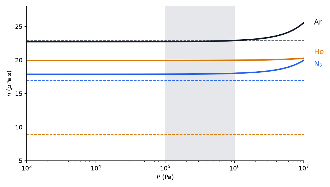
The viscosity of helium (orange), nitrogen (blue) and argon (black) at from to , from the NIST Chemistry WebBook’s reference correlations, with the kinetic estimate for each (dashed). Across the shaded decade from 0.1 to — a tenfold change of density — each changes by less than one per cent; nitrogen and argon rise by about by , where the gas is no longer dilute. Below the curves are flat by construction, the dilute-gas form the correlations assume.
Read the table honestly. The density independence is the robust prediction, and it holds. The estimates themselves are good to a factor of order one, and their near-perfect agreement for nitrogen and argon is partly luck: the careful theory’s coefficient is about 1.5 times the crude one (advanced section), and the van der Waals diameter happens to be smaller than a collision diameter by about the amount that compensates. For helium the two errors add, and the estimate is low by half. The ratio is the cleaner test, because the molecular size cancels from it: the crude estimates give exactly 1, and both monatomic gases give 2.51 — the careful theory’s — because the fastest molecules carry the most energy and also fly the furthest. The measured self-diffusion coefficients at and one atmosphere, (argon) and 1.72 to (nitrogen) (Winn 1950, Hutchinson 1949 and Winter 1951, as tabulated by Hirschfelder, Curtiss and Bird), are 1.3 and 1.4 times the estimates.
8. Against reality: Perrin’s atoms. Perrin’s 1909 memoir tabulates how many of the horizontal projections of 30-second displacements of gamboge granules, radius , fell between successive multiples of , as counted by his student Chaudesaigues for two series of fifty granules.
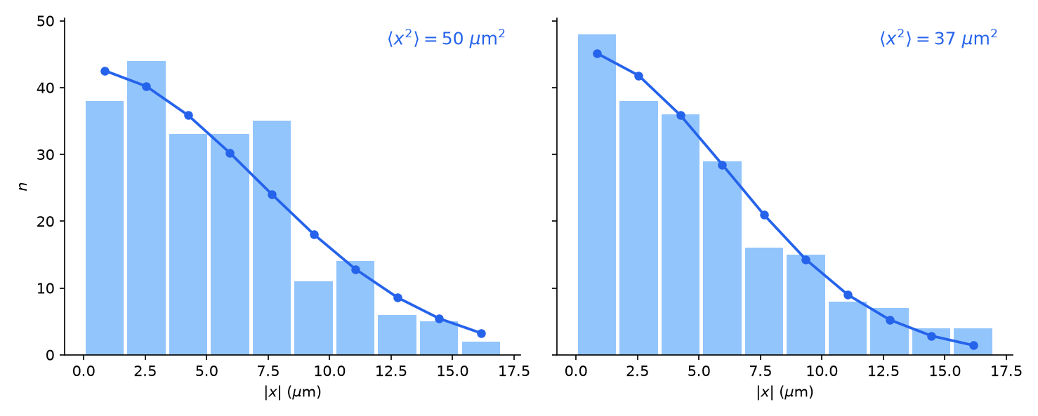
The sizes of the 30-second horizontal projections of gamboge granules, radius
, counted in bins of by Chaudesaigues for Perrin’s 1909 memoir
(bars): left, the first series, 221 projections in water at ; right, the
second, 205. The blue points are the Gaussian fitted to each table by fit_binned_gaussian_variance,
the estimator that measured the walkers’ histograms.
The fit to the first series gives , the error from resampling the table. So , and with the viscosity Perrin gives, 0.011 poise, the Stokes–Einstein relation turns it into
against the value fixed since 2019 by the definition of the mole, . The is the counting noise of 221 numbers and nothing else, and the table supports other honest readings: its second moment, taken from the bin centres, is , and its mean gives 45 — Perrin himself found 50.2 from the mean length of the displacements. The least-squares fit leans on one over-full bin (35 found between 6.8 and , where the fit expects 23). The three readings give from 6.5 to ; the second series, whose temperature Perrin does not give, fits to 37 against his 45. Two hundred and twenty-one numbers written down by hand in 1908 weigh an atom to within about , with a choice of estimator that matters as much as their counting noise. Perrin’s summary of seven displacement measurements (Atoms, 1916, p. 123) — granule radii from 0.21 to , masses differing fifteen-thousand-fold, viscosities more than a hundredfold — gives values from 5.5 to , with a mean of and a scatter of . A number that does not care what it is measured with is a property of the world.
The falsifying experiments. Each misconception this module confronts has a measurement above that it cannot survive. “Fluctuations in a simulation are numerical error, which a longer run would remove”: a thousandfold longer run left at (item 2), the value a heat capacity fixes, and the noise of a single temperature measured that heat capacity as well as heating did (item 1). “Diffusion carries particles at a steady speed”: the cloud’s width grew by 1.99 in four times the time (item 4), and a diffusion front’s position depends on alone (step 4). “A rarefied gas is less viscous”: a tenfold change of density moved the viscosity of nitrogen by (item 7).
Transfer the idea
One idea — that how far things spread, and how much they carry, is fixed by how long their motion is remembered — reaches back through the whole course and out into the world.
Back to module 03. The diffusion equation’s hypotheses are the central limit theorem’s: independent steps of finite variance. The persistent walk’s , which module 03 found in a variance, is here a Green–Kubo integral.
Back to module 04. Its model specification listed “high density (particle–particle collisions matter)” as a failure mode. This module put numbers on the collisions it left out — and — and measured the consequence: a gas without them never diffuses.
Back to module 08. A spreading cloud is entropy increasing in real time. A Gaussian of variance has an entropy per walker of , up to a constant fixed by the unit of length, which grows as without end until a wall stops it — the second law, watched.
Back to modules 11 and 12. The identity that module 12 derived became a measurement, and the equivalence of ensembles that module 11 found for one solid followed for any system with extensive and .
Back to module 13. Fick’s law is the dilute case of a more general rule: particles drift down the gradient of the chemical potential, . With module 13’s it is Fick’s law exactly; with interactions or an external potential it is not, which is how particles can flow towards higher concentration. The factor is the Einstein relation.
Back to module 15. Its autocorrelation time, the reason correlated samples are worth fewer independent ones, is a Green–Kubo sum: is the same arithmetic as .
Back to module 17. A metal conducts heat with its electrons, at the Fermi velocity rather than a thermal one. Step 8’s estimate with module 17’s electronic heat capacity per volume, , and copper’s measured conductivity of about gives an electron mean free path of about , a hundred atomic spacings.
Thermal noise in electronics. A resistor at temperature produces a fluctuating voltage whose mean square in a bandwidth is (Johnson and Nyquist, 1928): the electrical Einstein relation, with the resistance as the dissipation. It sets the floor of every sensitive amplifier, and has been used to measure .
Double glazing. The gap between two panes is filled with argon rather than air because argon conducts heat about less: its atoms are heavier and slower, and carry only translational energy. NIST’s values at , from item 7’s data, are 17.8 for argon and for nitrogen, the main part of air.
Biology. Diffusion supplies a cell in hundredths of a second and a millimetre of tissue in minutes, and would need months to cross a human body. Lungs, gills and blood vessels exist because diffusion is fast only over short distances.
Looking ahead — beyond this course:
Nonequilibrium statistical mechanics. Every result here assumed local equilibrium. Without it come Boltzmann’s transport equation, which follows the full velocity distribution of a gas; Onsager’s reciprocal relations, which tie together the coefficients of coupled flows; and Kubo’s linear response theory, of which the Green–Kubo relation for is the simplest case. The course ends at that door.
Worked examples
Try each one before opening its solution.
Worked example 1 — a heat capacity from the noise. A cluster of 1000 atoms in contact with a gas at has an energy that fluctuates with a standard deviation of . What is its heat capacity per atom, in units of ? What is the relative fluctuation of its energy, if ?
Solution
, which is per atom: Dulong and Petit, read off the noise. , so ; for a gram of the same solid it would be about 10-11.
Worked example 2 — what diffusion can supply. Oxygen in water has . How long does it take to spread across a cell wide, across , and across ?
Solution
: ; , about four minutes; , eight years. Tenfold the distance is a hundredfold the time.
Worked example 3 — a vacuum chamber. Estimate the mean free path of nitrogen at and , with , and the Knudsen number in a chamber across.
Solution
and , so and . A molecule crosses the chamber hundreds of times between collisions with other molecules: the gas has no viscosity in the sense of step 8, and its “flow” is molecules flying from wall to wall.
Worked example 4 — the viscosity of argon. Estimate the viscosity of argon at from step 8, with and the van der Waals diameter , and compare with the measured .
Solution
and , so . Within a per cent of the measurement — more closely than the method deserves, as item 7 of the verification explains.
Worked example 5 — a bead under the microscope. A bead of radius wanders in water at , viscosity . Find its , the root-mean-square displacement along one axis in , and the time it needs to wander .
Solution
. In , — five bead diameters, easy to see in a microscope. To wander it needs , about two weeks.
Check your understanding
A simulation of a small crystal in contact with a heat bath records its total energy, and the energy scatters by about 2% from sample to sample. A colleague proposes running the simulation ten times longer to make the scatter go away. What will the longer run do?
A. The scatter stays at about 2%; what shrinks, by about sqrt(10), is the uncertainty of the mean energy and of the scatter itself. B. The scatter falls by about sqrt(10), because random errors average out as one over the square root of the number of samples. C. The scatter falls by about a factor of 10, since ten times as many samples are averaged. D. The scatter grows, because a longer run accumulates more rounding error.
Check your answer
Correct answer: A — The scatter stays at about 2%; what shrinks, by about sqrt(10), is the uncertainty of the mean energy and of the scatter itself.
A. Right. The scatter is sigma_E = sqrt(k_B T^2 C_V), a property of a crystal on a bath: module 12’s identity. More samples measure it more precisely -- the standard error of the mean energy falls as one over the square root of the number of samples -- but they do not change it. In the laboratory, a thousandfold longer run left sigma_E at 8.80 gap while the error of the mean fell thirtyfold. The scatter is a heat-capacity measurement, not an error.
B. That is true of the uncertainty of the mean, not of the scatter. The standard deviation of the samples is a property of the distribution they are drawn from; the standard error of their average is that deviation divided by sqrt(n). The distribution here is the canonical one, whose width is sqrt(k_B T^2 C_V) however long it is sampled.
C. Averaging shrinks the uncertainty of an average as one over the square root of the number of samples, not as one over the number -- and in any case the scatter of the individual samples is not an average at all. It stays at sqrt(k_B T^2 C_V).
D. Rounding error in a sampler like this one is about one part in 10^16 per number and does not accumulate into a 2% scatter. The scatter is physical: draw the same crystal with its energy fixed (microcanonically) and it vanishes; put it on a bath and it returns, at exactly the size its heat capacity fixes.
One thousand independent two-level systems with gap Delta = 1.0e-21 J sit on a heat bath at T = 30.4 K. Their total energy is sampled many times and has a standard deviation of 8.80 Delta. What heat capacity per system does this imply, in units of k_B? (Give two decimal places.)
Check your answer
Correct answer: 0.44 (± 0.01)
C_V = sigma_E^2/(k_B T^2) = (8.80e-21 J)^2 / (1.381e-23 J/K x 30.4^2 K^2) = 7.74e-41 / 1.276e-20 = 6.07e-21 J/K for the thousand, or 0.44 k_B per system. Module 12’s closed form at Delta/(k_B T) = 2.38 gives k_B x^2 e^x/(e^x + 1)^2 = 0.439 k_B: near the top of the Schottky peak, measured from one temperature with nothing heated.
A canonical system of N independent subsystems has a relative energy fluctuation sigma_E/. You double N at the same temperature. What happens to sigma_E/, and what does that say about the canonical and microcanonical descriptions of a macroscopic body?
A. It falls by a factor sqrt(2) -- sigma_E grows as sqrt(N) while grows as N -- so for macroscopic N the energy is sharp and the two descriptions agree. B. It halves, because the fluctuations of independent subsystems cancel in proportion to their number. C. It does not change -- both sigma_E and are proportional to N. D. It grows by a factor sqrt(2), because a larger system has more energy to fluctuate.
Check your answer
Correct answer: A — It falls by a factor sqrt(2) -- sigma_E grows as sqrt(N) while grows as N -- so for macroscopic N the energy is sharp and the two descriptions agree.
A. Right. Var(E) = k_B T^2 C_V and C_V is extensive, so sigma_E grows as N^(1/2) while grows as N: the ratio goes as N^(-1/2). For a mole of two-level systems at k_B T = Delta it is 2e-12, and no measurement can tell an energy fixed exactly from one that fluctuates by a part in 10^12. That is the equivalence of ensembles.
B. Independent fluctuations do not cancel in proportion to their number; their variances add. N subsystems have N times the variance, so sigma_E grows as sqrt(N), and the ratio to falls as N^(-1/2): by sqrt(2) when N doubles, not by 2.
C. is proportional to N, but sigma_E is not: it is the variance that adds. If sigma_E grew in proportion to N, the relative fluctuation of a macroscopic body would be as large as that of a single molecule, and no thermometer would ever settle.
D. The absolute fluctuation sigma_E does grow, by sqrt(2). The relative one falls, because doubles. Large bodies look steady because the relative fluctuation is what an instrument sees.
A layer of dye at the bottom of a tall jar of set gelatin, in which nothing can flow, has one day after it was laid down coloured the gelatin up to 1 cm above the layer. How long after it was laid down will the same shade reach 2 cm?
A. 4 days -- every feature of a diffusion front advances as sqrt(D t), so twice the distance takes four times as long. B. 2 days -- the dye moves up at a steady 1 cm per day. C. About 1.4 days -- a diffusion front advances as t^2, faster and faster. D. 8 days -- the volume to be filled grows as the cube of the distance.
Check your answer
Correct answer: A — 4 days -- every feature of a diffusion front advances as sqrt(D t), so twice the distance takes four times as long.
A. Right. The dye-layer solution, c/c_0 = (1/2) erfc(x / (2 sqrt(D t))), depends on x and t only through x/sqrt(D t), so any contour of fixed shade sits at a fixed multiple of sqrt(D t). To double x, t must be multiplied by 4. In a jar of plain water the experiment rarely works: small temperature differences drive convection that carries the dye far faster. Gelatin stops the flow and leaves the diffusion.
B. Nothing in diffusion moves at a steady speed. A dye molecule does move fast -- over a hundred metres per second -- but its velocity is forgotten after about 1e-13 s, so its displacements add like a random walk’s, as sqrt(t). The front decelerates: it covered the first centimetre in a day and needs three more days for the second.
C. Spreading as t^2 is ballistic motion, which a molecule shows only for times shorter than its memory of its velocity -- about 1e-13 s in water. Over days the mean squared displacement grows as t, and distances as sqrt(t).
D. The jar is a one-dimensional problem: the dye spreads upward from a layer that fills the whole cross-section. Even for a point source in three dimensions the width of the cloud grows as sqrt(6 D t), so doubling a distance still takes four times as long.
On a log-log plot, the mean squared displacement of tracer particles has slope 2 at short times and slope 1 at long times. What does this tell you?
A. At short times the tracers move ballistically, x = v t, keeping their velocities; at long times their velocities have been randomised and they diffuse, <x^2> = 2 D t. B. The tracers move twice as fast at short times as at long times. C. At long times the tracers have slowed to a constant speed, because x grows linearly in t. D. The slope-2 part is a numerical artefact of having too few tracers.
Check your answer
Correct answer: A — At short times the tracers move ballistically, x = v t, keeping their velocities; at long times their velocities have been randomised and they diffuse, <x^2> = 2 D t.
A. Right. <x^2> = <v^2> t^2 while a velocity is remembered, slope 2; long after, the displacement is a sum of many independent pieces and grows as 2 D t, slope 1. The crossover marks the memory time -- for a gas, the time between collisions. The laboratory’s persistent walkers show both regimes in one curve.
B. A slope on a log-log plot is an exponent, not a speed. Slope 2 means <x^2> grows as t^2, slope 1 that it grows as t. The tracers’ speed does not change at all; what changes is whether their successive displacements are correlated.
C. Slope 1 means <x^2> grows linearly in t, so x itself grows as sqrt(t) -- no constant speed. Steady-speed motion would give slope 2, the short-time regime.
D. Too few tracers make the curve noisy, not steeper. Slope 2 at short times is physics: over times shorter than its velocity memory a particle simply flies. It is the regime module 04’s collisionless gas never leaves until it reaches a wall.
Treat nitrogen molecules as hard spheres of diameter d = 0.31 nm. At 0 C and one atmosphere the number density is n = 2.69e25 per cubic metre. Using lambda = 1/(sqrt(2) n sigma) with sigma = pi d^2, what is the mean free path, in nanometres?
Check your answer
Correct answer: 87 (± 5)
sigma = pi (0.31e-9 m)^2 = 3.02e-19 m^2, so lambda = 1/(1.414 x 2.69e25 x 3.02e-19) = 8.7e-8 m = 87 nm: about 280 molecular diameters and 26 mean spacings. With a mean speed of 454 m/s the collision rate is vbar/lambda = 5.2e9 per second. The diameter here comes from the van der Waals b, which module 02 obtained from the critical point; a diameter inferred from viscosity is about 20% larger, which is the honest size of the uncertainty.
A sealed container of nitrogen at room temperature and one atmosphere is pumped down to half an atmosphere, at the same temperature. What happens to the gas’s viscosity?
A. It stays the same -- half as many molecules carry momentum, but each flies twice as far between collisions. B. It halves -- with half as many molecules there is half as much to rub. C. It doubles -- the molecules fly twice as far between collisions. D. It falls by a factor sqrt(2), like the mean speed of a gas whose density is halved.
Check your answer
Correct answer: A — It stays the same -- half as many molecules carry momentum, but each flies twice as far between collisions.
A. Right. eta = (1/3) n m vbar lambda and lambda = 1/(sqrt(2) n sigma), so the density cancels: eta = m vbar/(3 sqrt(2) sigma). Maxwell predicted this in 1860 and confirmed it with swinging discs in 1866; NIST’s reference data for nitrogen at 300 K change by less than 1% between 1 kPa and 1 MPa. It fails only when the mean free path becomes comparable with the container, in a vacuum.
B. Gas viscosity is not rubbing. It is momentum carried across a plane by molecules flying from a faster layer to a slower one. Halving their number halves the carriers but doubles the distance each flies, so each brings twice the momentum difference. The two effects cancel exactly in the dilute gas.
C. The mean free path does double, but there are half as many molecules to fly it. The viscosity is the product of the two, and it does not change.
D. The mean speed of the molecules depends on the temperature alone, vbar = sqrt(8 k_B T/(pi m)), not on the density. At fixed temperature nothing in eta = m vbar/(3 sqrt(2) sigma) changes.
In three or four sentences: why are three independent measurements of a diffusion coefficient that agree within their error bars more convincing than one very precise fit? What would it have meant if one of them had disagreed with the other two by ten error bars?
Check your answer
The three use different features of the data -- the growth of the mean squared displacement (dominated by the cloud’s tails), the shape of the histogram (dominated by its middle), and the integral of the velocity autocorrelation (which uses no positions at all) -- and each rests on a different chain of assumptions. A single fit, however precise, can be wrong in a way its own error bar cannot show: a bias in the estimator, a non-Gaussian shape, a drift. Agreement across methods makes such hidden errors unlikely, because they would have to conspire. A disagreement by ten error bars would mean the methods are not measuring the same thing: for example, the histogram not Gaussian (too early, or steps of infinite variance), a drift adding to the mean squared displacement, or a cut-off of the velocity integral shorter than the memory. A strong answer adds that a two-error-bar difference in one run is not by itself a disagreement -- it happens about one time in twenty -- and that repeating the experiment under new seeds is how to tell bad luck from a bad method.
Every transport coefficient in this module assumes local equilibrium. Where does that description fail first?
A. Where the temperature, density or flow speed changes appreciably over a mean free path -- the Knudsen number lambda/L is not small, as in a vacuum chamber, a nanometre pore or a shock wave. B. At low temperature, because the molecules move too slowly to carry anything. C. At high density, because then the molecules collide too often to carry anything. D. Whenever there is any gradient at all, since a system with a gradient is not in equilibrium.
Check your answer
Correct answer: A — Where the temperature, density or flow speed changes appreciably over a mean free path -- the Knudsen number lambda/L is not small, as in a vacuum chamber, a nanometre pore or a shock wave.
A. Right. A parcel of gas has a temperature only if its molecules collide many times before meeting any appreciable change. When lambda/L is not small, molecules fly from wall to wall carrying conditions from far away, and viscosity and conductivity stop being properties of the gas. At 1e-4 Pa the mean free path of nitrogen is about a hundred metres, larger than any vacuum chamber.
B. Slow molecules still collide, and a cold dilute gas still has local equilibrium as long as its mean free path is short compared with its gradients. Cold matters only when quantum effects set in (module 17), which is a different failure.
C. Frequent collisions are what local equilibrium needs. A dense gas or a liquid is closer to local equilibrium, not further. What fails at high density is the dilute-gas estimate of the coefficients themselves -- molecules no longer fly freely between collisions -- not the assumption that each parcel has a temperature.
D. The whole system is not in equilibrium, but each small parcel can be, very nearly. That is the content of local equilibrium, and it holds whenever the gradients are gentle on the scale of a mean free path -- which at room conditions is 0.1 micrometre.
Two spherical beads, one twice the radius of the other, wander in the same water at the same temperature. How do their diffusion coefficients compare?
A. The larger bead’s D is half the smaller one’s -- the drag 6 pi eta a doubles, and D = k_B T / zeta. B. The larger bead’s D is an eighth of the smaller one’s, since it is eight times as heavy. C. They are the same -- D depends only on the temperature. D. The larger bead’s D is a quarter of the smaller one’s, since the drag on a sphere grows as its cross-sectional area.
Check your answer
Correct answer: A — The larger bead’s D is half the smaller one’s -- the drag 6 pi eta a doubles, and D = k_B T / zeta.
A. Right. The Einstein relation ties D to the friction coefficient, D = k_B T/zeta, and Stokes drag makes zeta proportional to the radius. The mass, which grows eightfold, does not enter: a heavier bead remembers its velocity longer but has a smaller thermal velocity, and the two compensate exactly.
B. Mass cancels out of D. Green-Kubo gives D = <v_x^2> tau_c with <v_x^2> = k_B T/m and tau_c = m/zeta: the heavier bead moves more slowly but keeps its velocity longer. Only the drag remains, and it grows as the radius.
C. The temperature sets the size of the kicks, but how far a kick carries a bead depends on how strongly the water resists it: D = k_B T/zeta, with zeta = 6 pi eta a.
D. For slow, smooth flow -- which a micrometre bead in water is, by a factor of a million -- Stokes drag grows as the radius, not as the area. Drag proportional to the area is the fast, turbulent regime of a falling raindrop.
A bead of radius 0.50 micrometres in water of viscosity 1.00e-3 Pa s at 293 K is tracked, and its displacements along one axis over 30 s have a mean square of 25.8 square micrometres. Using the Stokes-Einstein relation and R = 8.314 J/(mol K), what value of Avogadro’s number does this imply, in units of 1e23 per mole? (One decimal place.)
Check your answer
Correct answer: 6.0 (± 0.15)
D = <x^2>/(2t) = 25.8e-12 m^2 / 60 s = 4.30e-13 m^2/s. Then k_B = 6 pi eta a D/T = 9.42e-9 kg/s x 4.30e-13 m^2/s / 293 K = 1.38e-23 J/K, and N_A = R/k_B = 6.0e23 per mole. Perrin did this with gamboge grains in 1908-1909 and found values near 7e23; the gas constant came from balances and pressure gauges, so the beads weighed a molecule.
A walker steps +/-l every tau. With probability q = 0.5 it repeats its previous step, and otherwise it takes a fresh step, left or right with equal probability (module 03’s persistent walk). By what factor is its diffusion coefficient larger than the independent-step value l^2/(2 tau)?
Check your answer
Correct answer: 3 (± 0.05)
Its velocity is correlated with the one k steps later by q^k (a fresh step is uncorrelated with everything before it), so the Green-Kubo sum is tau (l/tau)^2 (1/2 + q + q^2 + ...) = (l^2/(2 tau)) (1 + q)/(1 - q) = 3 l^2/(2 tau). The formula l^2/(2 tau) assumed independent steps; with memory it is wrong by exactly the factor module 03 found in the persistent walk’s variance.
Exam-style problems for this module — the ones worth doing with a pen — are collected in the problem set.
Explain it in your own words
Answer in a few sentences each.
A skeptic says that the energy fluctuation in a simulation is numerical error and will vanish if the simulation is run long enough. Convince them otherwise, using a measurement they could make.
A dye front slows down as it advances, although nothing slows the molecules. Explain why.
Why does removing half of a gas leave its viscosity unchanged? Explain it in terms of what a single molecule does.
The course began by asking how macroscopic order emerges from microscopic chaos. In what sense does this module say the chaos is not merely tolerated by the order but does the work?
Advanced: the Green–Kubo relation, and the careful coefficients
Where the Green–Kubo relation comes from
Write the displacement as the integral of the velocity and square it:
In a steady state the correlation depends only on the separation, , and is even. The integrand is constant along every diagonal of the square , and the diagonal at separation has length proportional to , so
At short times and . At long times the slope tends to , which is , provided the integral converges — provided the memory dies faster than . For velocities that are constant over steps of length the same argument, with sums for integrals, gives exactly: the trapezoid rule is no approximation there, which is why the laboratory’s third estimate needs no correction.
The proviso is not a formality. In 1970 Alder and Wainwright found, in computer simulations of hard disks and spheres, that a tagged particle’s velocity memory in a dense fluid does not die exponentially: it decays as a power, in dimensions, because the particle’s own momentum, shared with the fluid around it, comes back to it as a slowly spreading vortex. In three dimensions is integrable and exists. In two it is , the integral diverges logarithmically, and a two-dimensional fluid strictly has no diffusion coefficient at all.
The persistent walk, exactly
For module 03’s persistent walk, , and the double sum can be done in closed form:
For it is , ballistic; for it is a straight line of slope
with , offset below the origin by . That
offset is why d_from_msd fits the slope of the late-time line with a free intercept rather than
dividing by , and why d_from_histogram fits the growth of the variance
between snapshots rather than its value at one. The crossover from slope 2 to slope 1 sits at
about twice the memory time : for the log-log slope falls through 1.5 at
21 steps.
What the careful theory changes
Step 8’s argument gives every molecule the mean speed and the mean free path. Chapman and Enskog, solving Boltzmann’s transport equation for hard spheres to first order, gave the careful results:
At the same diameter these are 1.47, 3.7 and 1.77 times step 8’s estimates. The viscosity keeps its independence of the density; the thermal conductivity’s extra factor — the measured 2.51 of item 7 for helium and argon — comes from the fastest molecules carrying both the most energy and the longest flights. Fitted to the measured viscosity at , the Chapman–Enskog formula gives hard-sphere diameters of for helium, for nitrogen and for argon, against the van der Waals values 0.266, 0.313 and — larger for nitrogen and argon, smaller for helium. A molecule has no single size. The van der Waals is fitted at the critical point, where the attraction between molecules matters as much as their repulsion; the viscosity probes the repulsive core in collisions at room-temperature energies. Neither is a hard-sphere diameter, because molecules are not hard spheres, and each measurement of reports the size its own process sees.