Phase transitions and the Ising model
The puzzle: who chooses the direction?
Hold a magnet in a flame and it stops being a magnet. Iron loses its magnetization at , its Curie temperature, and the loss is not a slow fading: just below that temperature the iron is magnetized, just above it is not, and the magnetization goes to zero continuously but with a vertical tangent. Let it cool again and, at the same temperature, the magnetization comes back.
It has to come back pointing somewhere. And here is the trouble. The energy of a piece of iron in zero field does not care which way its moments point, as long as neighbours agree: flip every moment in the sample and the energy is exactly what it was. The equations are symmetric between “up” and “down”. The sample, cooled through its Curie point, is not — it picks one.
Module 14 left a second question at the same place. Its coexistence curve ended: at the critical point the latent heat vanished and the liquid and gas densities merged as , while real fluids merge as , an exponent the van der Waals model cannot produce. This module answers both with one model, so simple it fits in a line, and with a computer experiment: the Ising model and the Monte Carlo method. Along the way it asks what a simulation of 4096 spins can and cannot tell us about a transition that, strictly, only happens in an infinite system.
Predict before you calculate
Commit to an answer for each of these before reading on. Write them down.
A large square lattice of spins is cooled far below its transition temperature in zero field. In equilibrium, is its magnetization zero, close to , or does it depend on how it was cooled?
A computer samples the lattice’s equilibrium at three temperatures: well below the transition, at it, and well above it. At which temperature does the simulation take the longest to forget where it started?
The magnetization is computed against temperature for lattices of side 16 and 64. Which curve drops more sharply at the transition?
Below the transition, a field is swept slowly from strongly up to strongly down and back. Does the magnetization retrace the same curve on the way back, or not?
Explore the model
The laboratory runs a live Ising lattice. You set the temperature, the field and the size, watch the spins, and read the magnetization and energy traces as they are produced. Then it runs the experiments this module is built on: a one-dimensional chain against its exact solution, a temperature sweep for three sizes with the susceptibility and heat capacity read from fluctuations, a measurement of how long the simulation takes to decorrelate, a field swept up and down below and above the transition, and the same lattice run under two different update rules.
A lattice quenched from infinite temperature to , well below the transition. Left: the spins, up dark and down light. Within a few sweeps the random speckle organises into domains of each sign; then the domains coarsen, the small ones shrinking and the large ones growing, because every boundary costs energy. Right: the absolute magnetization per spin (blue) and the energy per spin (red), against the number of sweeps on a logarithmic axis — each sweep offers every spin one chance to flip. The energy is nearly settled within a hundred sweeps, because the domain walls are by then a small fraction of the bonds. The magnetization is not: with large domains of both signs it stays near zero for two thousand sweeps, until the last band of light spins narrows and closes and jumps to the grey dashed line, the exact equilibrium value for the infinite lattice. In about one run in four at this size the lattice instead freezes into two straight bands, one of each sign, which outlast this window by far. Nothing chose which sign wins except the random history of the run.
Run the laboratory now, then come back. Four things are worth doing before you read on:
Set and run a lattice from a random start, then from an all-up start. Then set and do the same. Which runs end up in the same place?
Set the temperature just below and watch the magnetization trace. Then set it just above. Compare how long the trace takes to wander across its range.
Run an lattice at for a long time and watch the sign of the magnetization. Then a lattice at the same temperature.
Sweep the field from +1 to -1 and back at , then at .
Derive the result
System and boundary. spins on a lattice, each or -1, held at temperature by a bath and subject to a uniform external field , measured as an energy per unit spin. The lattice is periodic. The spins are classical: is a number, not an operator.
Independent variables. The temperature and the field ; the configuration is a microstate, and the energy , the total spin and the magnetization per spin are functions of it.
Sign convention. The course convention, , holds and is not exercised: nothing in this module computes a heat or a work. The heat capacity enters only through module 12’s fluctuation identity, which needs no sign convention.
Units. This module measures energies in units of , temperature as and field as . Critical behaviour is the one subject in the course where the material constants genuinely scale out — that is what universality, below, claims — and stays in every formula through . To quote a number for a material, put and back: a coupling of puts the square lattice’s transition at .
Route. Six steps. Write the model and its symmetry; derive the Monte Carlo rule from module 11’s Boltzmann distribution; show that one dimension cannot order; build the mean-field theory of module 12’s paramagnet with an effective field; state Onsager’s exact answer in two dimensions and measure how wrong mean field is; and read the critical behaviour from module 12’s fluctuation identities.
Step 1: the model, the order parameter, and the symmetry
A bond costs when its two spins agree and when they disagree. The ground state at is all spins aligned, with — on the square lattice, bonds and . There are two ground states, all up and all down, and they have the same energy.
At the energy is invariant under flipping every spin, for all , because each bond energy depends on the product . So the Boltzmann weight of a configuration and of its flipped twin are equal, , while their magnetizations are opposite. Pairing every configuration with its twin,
This is exact, and it is the puzzle sharpened. For any finite lattice, the canonical average of the magnetization in zero field vanishes at every temperature. If there is a magnetized phase, it cannot be found by computing at for finite .
What is computable is how the average responds to a small field, and in which order the limits are taken:
The order of limits is the whole content. Take first at finite and the answer is zero, by symmetry. Take first, and below the transition an arbitrarily weak field — a stray field, a single defect, the history of the sample — is enough to tip the whole system one way. That is who chooses the direction: the system’s own history, amplified by its size.
The finite- version of the same story is told in time rather than in limits. Below the transition, a finite lattice in zero field does occasionally reverse its magnetization: it must, or the average would not be zero. But to reverse, it has to pass through configurations with a wall of reversed spins running all the way across it, which costs an energy that grows with , so the waiting time between reversals grows exponentially with the system’s size. For a magnet of 1020 spins it exceeds the age of the universe. The ensemble average is zero; the sample, for every practical purpose, is not. This is ergodicity breaking: the dynamics no longer explores all the states the ensemble averages over.
Step 2: Monte Carlo from detailed balance
To see any of this, we need the canonical averages of a lattice of thousands of spins. The partition function of a lattice is a sum of 24096 terms, and no closed form exists outside special cases. The way around it is to sample: generate configurations with the right probability and average over them.
Module 11 established the target. In equilibrium with a bath at temperature , a configuration occurs with probability
Build a random walk through configuration space: from the current configuration , propose flipping one spin, giving , and accept the proposal with some probability . Proposals are symmetric — choosing which spin to flip does not depend on the state. We want the walk, run for long enough, to visit each configuration with probability . A sufficient condition is that in equilibrium the flow from to balances the flow back, for every pair:
Check the rule in both cases. If , then and the reverse move lowers the energy, so : the ratio is right. If the roles swap and the ratio is , right again. Stationarity follows by summing detailed balance over : , since the walk must go somewhere. The partition function never appears: only ratios of Boltzmann weights do, which is why sampling succeeds where summation is hopeless.
For the Ising model the energy change of flipping spin needs only its neighbours. Writing for the sum over the neighbours of site ,
On the square lattice at it takes only five values, , , 0, and .
One practical point decides whether the method is right or wrong. Updating every spin at once, each against the configuration before the update, breaks detailed balance: two neighbours that both flip each computed against a neighbour that no longer exists. The laboratory colours the lattice like a chessboard instead. Every neighbour of a black site is white, so with the white sites held fixed the black sites do not interact, and updating all of them at once is the same as updating them one at a time. A sweep is a black half-sweep followed by a white one. Each half-sweep satisfies detailed balance, so each leaves the Boltzmann distribution unchanged, and so does the sweep.
Step 3: why a chain cannot order
Start a ring of spins all up at . The cheapest way to destroy its order is a domain wall — a single bond whose two spins disagree, separating a block of up spins from a block of down. On a ring walls come in pairs; take two, cutting the ring into two arcs. Each wall costs , so two cost , independent of where they are. But the first can sit at any of bonds and the second at any of the others, roughly placements, each a distinct microstate. In module 08’s terms, the multiplicity of the two-wall states is about and their entropy is . The free energy cost of breaking the order is
The energy is fixed; the entropy grows without bound as grows. For any there is an beyond which , walls appear spontaneously, and the order is destroyed. The same accounting for a single wall in an open chain gives the form usually quoted, .
These two formulas are the module’s first exact anchors: the laboratory’s chain must reproduce them, within its error bars, before anything it says about two dimensions is believed.
The argument fails in two dimensions, and the way it fails is instructive. A wall that cuts a square lattice in two has a length of at least , so its energy cost grows like . Its entropy grows like too — a wall is a path, and a path of length can wander in at most ways — so energy and entropy now compete on equal terms, and at low enough temperature the energy wins. The argument does not prove that the square lattice orders; it shows that nothing like the one-dimensional catastrophe forbids it. Problem 2 makes it quantitative.
Step 4: mean field, and what it gets wrong
Module 12 solved a single spin in a field exactly: its average is . A spin in the Ising model feels the field plus its neighbours. The mean-field approximation replaces each neighbour by its average, so that spin sees an effective field
and responds to it as module 12’s paramagnet. Consistency demands that the average it produces be the that was assumed.
Just below , is small, and turns the equation into , so that
The magnetization vanishes as the square root of the distance to : exponent , the same exponent the van der Waals model gave module 14 for . That is not a coincidence. Both are mean-field theories — every particle, or every spin, feels the average of the others — and every mean-field theory gives .
Mean field is a good guess far from and a bad one near it, and it is worst in low dimensions. It predicts a transition for the chain, at , where step 3 proved there is none. For the square lattice it predicts . The exact answer is next.
Step 5: Onsager’s exact answer
In 1944 Lars Onsager solved the two-dimensional Ising model in zero field exactly. The derivation is one of the great calculations of theoretical physics and lies outside this course; its results are the module’s reference values.
So mean field overestimates the transition temperature by a factor , or . Its error is not one of detail. Near a spin’s neighbours are not an average — they are correlated with it and with each other over long distances — and mean field throws away exactly those correlations. And the exponent is not : Onsager–Yang’s vanishes as , far more steeply.
Step 6: critical behaviour, read from fluctuations
At the transition the system is neither ordered nor disordered: it is a patchwork of domains of every size, from single spins to the whole lattice. That is what makes responses diverge, and module 12’s fluctuation identities are how a simulation sees it.
Below , a finite run does not sample the two branches fairly — it crosses between them rarely, at a rate that depends on how long the run happened to be — so of a run measures luck. The laboratory applies the same identity to , which a run can sample, and reports . It is the standard estimator for finite lattices. Its peak is all the module uses.
Near the singular parts of the observables follow power laws in , with critical exponents conventionally called , , and (the first has nothing to do with ; context always tells them apart):
where is the correlation length, the size of the largest correlated patches. For the square lattice, from Onsager’s solution, , , , and the heat capacity diverges logarithmically (). Mean field gives , , and a finite jump in .
Three facts about these divergences decide what a simulation can see:
Nothing diverges on a finite lattice. cannot exceed , so on an lattice every peak is rounded and finite, its height grows with , and its position drifts toward as grows. The singularity at is a property of the limit .
The transition is continuous. Crossing at , the energy per spin is continuous — there is no latent heat, unlike module 14’s boiling — and the heat capacity peaks instead. Crossing below , by contrast, the magnetization jumps from to : a first-order transition, the magnetic version of boiling, along a line that ends at the critical point.
Critical slowing down. A local update rule changes a configuration one spin at a time, and a correlated patch of size takes a time that grows like to rearrange, with for Metropolis. At on a finite lattice , so the autocorrelation time grows like : the simulation is slowest exactly where the physics is most interesting.
Three lattices, (amber), 32 (red) and 64 (blue), drawn at the same size and cooled together from to through 41 temperatures. Top: the spins at each step. Bottom: for each lattice, added point by point as the temperature falls (temperature decreases to the right), against Onsager–Yang’s exact curve for the infinite lattice (black); the dashed line is . Above each lattice keeps a small residual , largest for the smallest lattice — a finite patch of random spins is never exactly balanced. Near the lattices fill with patches of both signs at every size up to the lattice itself. Below, all three order and their curves merge with the exact one. The rise is steepest for the largest lattice, and no finite lattice reproduces the black curve’s vertical drop.
The last one sets the standard for every number this module reports. A trace of samples whose autocorrelation time is (in samples) contains about
independent samples, and its standard error is , not . This is module 03’s correlated walk again: the law survives, with replaced by the number of samples that are actually independent. The laboratory measures as the integrated autocorrelation function, , summed out to a window several times itself.
The dictionary between the two problems is direct. Divide a fluid into cells, each occupied by a molecule () or empty (), with an attraction between occupied neighbours: that is an Ising model, the lattice gas. The magnetization is the density measured from its critical value, the field is the chemical potential, the line below is the coexistence curve, and the jump in across it is the jump from gas to liquid density.
Verify computationally
Every number below comes from thermolab.ising, run under several independent seeds, with every
error bar computed from the effective number of independent samples rather than the raw count.
The laboratory repeats each experiment at a smaller scale.
1. The bookkeeping. The simulation never recomputes the energy: each accepted flip adds its to a running total. After 1000 sweeps of a lattice at — tens of thousands of accepted flips — the running energy and total spin equal a from-scratch recount exactly, as integers. In a field the energy carries and agrees to rounding.
2. The chain against its exact solution. A 1024-site ring, eight seeds, 2000 sweeps each after 300 of burn-in, under the Glauber rule. At and the energy per spin is against the exact ; at , against -0.46212. In a field at the magnetization is against the exact 0.91382. All within one standard error. Under the Metropolis rule the same ring forgets a cold start far more slowly — after 100 sweeps of burn-in it still sits four standard errors low — because at in one dimension every wall move costs nothing and Metropolis accepts all of them, so the walls are pushed one way like beads on a wire instead of diffusing. Both rules reach the same answer eventually: a statement about speed, not about equilibrium.
3. Below , against Onsager–Yang. A lattice, six seeds: at , 2.0 and , , and , against the exact infinite-lattice 0.9865, 0.9113 and 0.7848. Below a lattice is already, to three decimals, infinite; the finite-size effects live near . Mean field at says 0.958.
4. Far above , against the high-temperature series. At in a weak field, a free spin would give . The square lattice’s high-temperature series gives , with . The simulation agrees with the series and rejects the free spin by many standard errors: even at ten times the neighbours still matter at the level.
5. The transition, located. The figure below is the module’s central measurement.
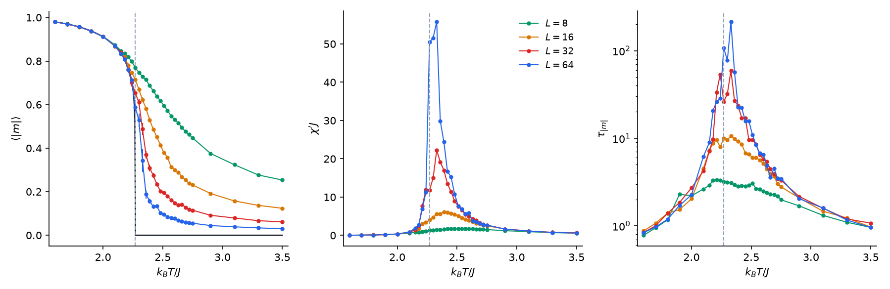
The square lattice at (green), 16 (amber), 32 (red) and 64 (blue), each point from one run of sweeps after burn-in at , falling to 5000 at ; the dashed line is Onsager’s . Left: with -corrected error bars, and Onsager–Yang’s exact curve for the infinite lattice (black). Below every size agrees with it; above, every finite lattice keeps a residual that falls with , and the shoulder sharpens without ever becoming the black curve’s vertical drop. Middle: the susceptibility , whose peak grows with and moves toward from above. Right: the autocorrelation time of , in sweeps: about one deep in either phase and peaking at , higher for every larger lattice — critical slowing down. The jagged points near the top of the right and middle panels are honest: at a run of 5000 sweeps holds only some 25 to 50 autocorrelation times there, and its fluctuation estimates scatter accordingly.
6. Critical slowing down, measured. On a lattice (four seeds of sweeps each), the autocorrelation time of is 0.7 sweeps at , 2.8 at 2.0, 41 at 2.27, 11.5 at 2.5, 1.7 at 3.0 and 1.0 at 3.5. At itself it grows with the lattice: 3.1, 9.6, 42 and sweeps at , 16, 32 and 64 — a power with fitted , near the value that large-scale studies of local update rules find. The settling time is largest at the transition, not anywhere near either side of it, and every doubling of quadruples it.
7. Who chooses the direction, measured. At , from an all-up start, run for 105 sweeps: an lattice reverses its magnetization 42 times, its time average of is 0.11, and its is 0.911. A lattice and a lattice never reverse: their time averages are 0.912 and 0.911, the spontaneous magnetization. At , closer to , the three lattices reverse 383, 52 and 3 times. The ensemble average of is zero for all of them; how much of the ensemble one run actually visits collapses as the system grows.
8. Hysteresis. A lattice, field stepped in 81 steps, four seeds. At the area of the loop is , and for 5, 20 and 80 sweeps per step: slower sweeps shrink it, and it stays open. At , 0.98, 0.51 and 0.27: still open, and narrowing faster. At , above , 0.013, 0.015 and 0.021, which is noise: the curve retraces itself.
A lattice at while the field is stepped from +1 to -1 and back, 20 sweeps per step. Left: the spins. Right: against ; the red dot is the current state and the blue curve its history. The magnetization keeps its sign well past — the state with in a negative field is metastable, module 14’s superheated liquid in magnetic form — until a reversed domain large enough to grow happens to form, and then the whole lattice reverses in a few frames. The grey curve is the same sweep at , above : one smooth curve through the origin, the same in both directions.
9. Two update rules, one equilibrium. Quench a random lattice to under each rule, eight seeds: after 5, 20 and 100 sweeps the energy per spin is -1.581, -1.804, -1.920 under Metropolis and -1.434, -1.675, -1.806 under Glauber. Glauber is visibly slower. At in equilibrium (, eight seeds), the two give and : the same answer, within 1.6 combined standard errors. How fast the chain gets there is the algorithm’s; where it gets to is the Boltzmann distribution’s.
10. The error bar itself. Sixteen independent runs at on a lattice, each reporting with its -corrected standard error: the average reported error matches the actual scatter of the sixteen means, while the naive is less than half of it. The test suite asserts both.
The falsifying experiments. Each misconception this module confronts has a measurement above that it cannot survive. “The system settles fastest at ”: item 6, where is largest exactly there and grows with . “Below the magnetization is zero because up and down cancel”: item 7, where every lattice large enough to be a magnet holds one sign for the whole run, and item 8, where the reading depends on the history. “Monte Carlo shows the real time evolution”: item 9, where two equally valid rules take different numbers of sweeps to reach the same equilibrium.
Against reality. No experiment on a bench pairs with this model: exchange couplings are invisible, and no cheap apparatus reaches a clean magnetic transition. Iron’s Curie temperature is and nickel’s , and the measured magnetization of both vanishes continuously, with a vertical tangent, as the module says it must. But neither is a two-dimensional Ising magnet: they are three-dimensional, and their moments can point in any direction, not just up or down. Their measured exponent lies near 0.36–0.38 — not the square lattice’s , not mean field’s , and not even the three-dimensional Ising value 0.326. Which class a system falls into is decided by the dimension and the symmetry of its order parameter, which is the content of universality.
Transfer the idea
The Ising model is the simplest system with a phase transition, and the Metropolis algorithm the simplest way to sample a distribution you cannot sum. Both travel far.
Back to module 11. The Metropolis rule is module 11’s Boltzmann distribution turned into an algorithm: the finite-bath argument said what the probabilities are, detailed balance says how to produce configurations with those probabilities one flip at a time.
Back to module 12. The fluctuation identities were reused unchanged — and are variances — and the limit of the Ising model is module 12’s paramagnet, exactly. Problem 6 recovers it.
Back to module 14. The field-driven reversal below is a first-order transition, with metastable states, nucleation and hysteresis — the magnetic version of the superheated liquid — along a line that ends at a critical point. Through the lattice gas the line is a coexistence curve, and the Ising critical point is a liquid–gas critical point. That is why module 14’s van der Waals exponent was wrong and the real fluid’s 0.32 is the Ising one.
Back to module 03. The autocorrelation time is the correlated walk’s lesson made quantitative: correlated samples still obey the law, but with replaced by , and an error bar that ignores it is too small by .
Forward to module 18. How long a fluctuation takes to die away — the correlation time — returns there as the time-correlation function of a transport process.
Critical opalescence. A fluid at its critical point turns milky. Its correlation length, the size of the correlated density patches, grows past the wavelength of light, and the patches scatter it — the same divergence the susceptibility peak reports here.
Magnetic memory. A bit on a hard disk is a small magnetized region whose reversal requires a field above its coercive field — the corner of the hysteresis loop. It keeps its bit for years because, like the large lattice of item 7, reversing it means crossing a barrier that grows with its size.
Monte Carlo everywhere. The same algorithm, with a different “energy”, samples the posterior distributions of Bayesian statistics (where it is called Markov chain Monte Carlo), folds proteins in simulation, and — with the temperature slowly lowered, “simulated annealing” — finds good solutions to optimization problems far too large to search. In every one of those, the autocorrelation time decides how much the output can be trusted.
Looking ahead:
Module 16 puts quantized energy levels into solids and radiation; its heat capacities are the smooth, transition-free cousins of this module’s peak.
Module 17 finds a phase transition with no interactions at all: Bose–Einstein condensation, driven by quantum statistics alone.
Module 18 asks how fluctuations relax in time, with the correlation time as its central quantity.
Worked examples
Try each one before opening its solution.
Worked example 1 — acceptance at the critical point. On the square lattice at and , find the Metropolis acceptance probabilities for flips with and , and the Glauber probability for .
Solution
Metropolis: and . (In fact exactly, from Onsager’s formula, so the first is .) Glauber: , lower, as it is for every . Both satisfy detailed balance; Glauber also accepts a flip only half the time, where Metropolis always does.
Worked example 2 — domain walls in a chain. For a ring at , how many sites must it have before two domain walls lower its free energy? How far apart are the walls actually, in equilibrium?
Solution
requires , so : about ten sites. The exact energy per spin means a fraction of the bonds are walls — one every 8.4 bonds. The two estimates agree on the scale: at order survives over a handful of sites, and no further.
Worked example 3 — mean field above the true transition. Solve the mean-field equation for the square lattice at and by iteration, starting from . What is the true spontaneous magnetization at this temperature?
Solution
Iterate : 0.583, 0.651, 0.700, 0.732, 0.752, , converging to 0.776. Mean field says the lattice is strongly magnetized. In truth is above Onsager’s , and . Mean field ignores the fluctuations that, at this temperature, destroy the order it predicts.
Worked example 4 — a heat capacity from a variance. A lattice at gives an energy-per-spin trace with variance . Find the heat capacity per spin.
Solution
; in reduced units . No derivative was taken: the response to heating is read off the spontaneous fluctuations, exactly as in module 12.
Worked example 5 — an honest error bar. A trace of 5000 samples of has standard deviation 0.08 and autocorrelation time 40 samples. Quote the mean’s standard error, and the naive one.
Solution
, so the error is . The naive is nine times too small — the factor . A result quoted with the naive bar would claim a precision the run does not have.
Worked example 6 — reading Onsager–Yang. Compute the exact spontaneous magnetization at .
Solution
; ; ; and . The simulation gives ; mean field gives 0.958.
Check your understanding
The Ising energy is E = -J sum_ s_i s_j - h sum_i s_i with J > 0. At h = 0, which statement about its symmetry and the order parameter m = (1/N) sum_i s_i is correct?
A. Flipping every spin leaves E unchanged and reverses m, so every canonical average of m vanishes at h = 0 for any finite N; an ordered state must pick one sign the equations do not prefer. B. J > 0 favours spins pointing up, so the h = 0 ground state is all up and m = +1. C. m measures the energy per spin, so it is zero whenever E is zero. D. The symmetry holds only above T_c; below T_c the energy itself prefers one sign.
Check your answer
Correct answer: A — Flipping every spin leaves E unchanged and reverses m, so every canonical average of m vanishes at h = 0 for any finite N; an ordered state must pick one sign the equations do not prefer.
A. Right. Each bond energy depends only on the product s_i s_j, so the all-flipped twin of any configuration has the same Boltzmann weight and the opposite m. The average over the pair is zero. Order appears only as spontaneous symmetry breaking: in the limit N -> infinity an infinitesimal field selects one branch.
B. J > 0 favours neighbours that agree, whichever way they point. All up and all down have exactly the same energy, -2NJ on the square lattice. Only a field h breaks the tie, and at h = 0 there is none.
C. m counts spins, not bonds. A checkerboard of alternating spins has m = 0 and the highest possible energy, +2NJ; an all-up lattice has m = 1 and the lowest. The order parameter and the energy are different functions of the configuration.
D. The energy function does not depend on the temperature at all, and its up-down symmetry holds at every T. What changes below T_c is not the equations but the state the system settles into.
A Metropolis simulation proposes a spin flip that would raise the energy by DeltaE = 4J, at temperature k_B T = 2J. With what probability is the flip accepted?
Check your answer
Correct answer: 0.135 (± 0.002)
A = min(1, e^(-DeltaE/(k_B T))) = e^(-4J/2J) = e^(-2) = 0.135. A move that lowers the energy would be accepted with probability 1. If you answered 0.0183, you used e^(-4); if 0.5, you halved the energy rather than exponentiating it.
A simulation reports that a 64 x 64 lattice quenched below T_c took about 2000 Metropolis sweeps to order. What does one sweep correspond to physically?
A. Nothing fixed. A sweep is one flip attempt per spin, a unit of computation; another rule with the same stationary distribution (Glauber) relaxes at a different speed to the same equilibrium. B. About one picosecond, the time a real spin takes to flip; multiply by 2000 to get the real ordering time. C. One period of the lattice vibrations that carry heat to the spins. D. The time for the field to propagate across the lattice at the speed of light.
Check your answer
Correct answer: A — Nothing fixed. A sweep is one flip attempt per spin, a unit of computation; another rule with the same stationary distribution (Glauber) relaxes at a different speed to the same equilibrium.
A. Right. Detailed balance fixes where the chain goes, not how fast. The laboratory runs Metropolis and Glauber side by side: the equilibrium energies agree within error, and the relaxation curves do not. The order of the domains forming is suggestive, but the clock is the algorithm’s.
B. This is the misconception that Monte Carlo simulates the real magnet’s motion. No physical constant converts sweeps into seconds: the update rule was chosen to sample the Boltzmann distribution, and a different valid rule gives a different number of sweeps for the same physics.
C. The model ignores lattice vibrations entirely; the bath is implicit. Nothing in the chain knows about phonons, so nothing in it can be timed by them.
D. Nothing propagates in the model. Each flip depends only on the current state of its neighbours, and the order in which sites are visited is a free choice of the algorithm.
Why does the one-dimensional Ising chain have no ordered phase at any T > 0, while the square lattice orders below 2.269 J/k_B?
A. In 1-D a domain wall costs a fixed energy 2J but can sit at any of N places, so its free energy 2J - k_B T ln N turns negative for large N at any T > 0; in 2-D a wall across the lattice costs energy proportional to its length, which can beat its entropy at low T. B. The coupling J is weaker in one dimension. C. The chain does order, but at a temperature too low to simulate. D. A chain has fewer spins, so fluctuations are larger.
Check your answer
Correct answer: A — In 1-D a domain wall costs a fixed energy 2J but can sit at any of N places, so its free energy 2J - k_B T ln N turns negative for large N at any T > 0; in 2-D a wall across the lattice costs energy proportional to its length, which can beat its entropy at low T.
A. Right. Entropy grows with the system and the 1-D wall’s cost does not, so walls always win and destroy long-range order. In 2-D, energy and entropy both scale with the wall’s length, and the energy wins below a temperature of order J/k_B.
B. J is the same bond energy in both. The difference is geometric: in 1-D one broken bond splits the system in two, while in 2-D splitting it takes a whole line of broken bonds.
C. The exact solution has m = 0 at every T > 0 in zero field: E/(NJ) = -tanh(J/(k_B T)) is smooth all the way down. Mean field predicts a transition at k_B T = 2J for the chain, and that prediction is simply wrong.
D. A chain can have as many spins as you like; the argument is about N -> infinity. What matters is how the cost of breaking the order scales with the system, not how many spins there are.
Mean-field theory gives k_B T_c = qJ = 4J for the square lattice; Onsager’s exact result is 2J/ln(1 + sqrt(2)) = 2.269J. By what percentage does mean field overestimate T_c?
Check your answer
Correct answer: 76.3 (± 0.5)
(4 - 2.269)/2.269 = 0.763, a 76% overestimate. Mean field replaces each neighbour by its average and so discards the correlations that, near T_c, decide everything. For the chain (q = 2) it is worse than inaccurate: it predicts a transition at 2J/k_B where there is none. If you answered 43.3, you divided by 4 instead of by the exact value.
A 32 x 32 lattice above T_c, at k_B T = 2.5 J, gives a magnetization trace with variance Var(m) = 0.0049. Using chi = N Var(m)/(k_B T), in units where J = 1, what is the susceptibility per spin?
Check your answer
Correct answer: 2.01 (± 0.03)
N = 32^2 = 1024, so chi = 1024 x 0.0049 / 2.5 = 2.01. This is module 12’s fluctuation identity: the response to a field is the size of the spontaneous fluctuations without one. If you answered 0.0628, you used N = 32 instead of 32^2.
A Metropolis simulation of a 32 x 32 lattice is run at k_B T = 1.5 J, 2.27 J and 3.5 J. At which temperature does the magnetization trace take the longest to decorrelate?
A. At 2.27 J, near T_c -- the autocorrelation time peaks there, and grows with L (critical slowing down). B. At 2.27 J it decorrelates fastest, since the system is between phases and neither holds it back. C. At 1.5 J, because the low temperature makes flips rare. D. At 3.5 J, because high temperature means large fluctuations.
Check your answer
Correct answer: A — At 2.27 J, near T_c -- the autocorrelation time peaks there, and grows with L (critical slowing down).
A. Right. At T_c the lattice is a patchwork of correlated domains of every size up to L, and a local rule rearranges a domain of size xi in a time that grows like xi^z with z near 2. The laboratory measures tau of |m| at about 1 sweep deep in either phase and tens of sweeps at T_c.
B. This is the misconception the slowing-down measurement falsifies. Being between phases means domains of both signs at every scale, and large correlated domains are the slowest thing a local update can change. tau peaks at T_c and keeps growing with L.
C. Flips are rare deep in the ordered phase, but |m| has almost nothing to do: it sits near 0.99 with tiny independent fluctuations, so its trace decorrelates within a couple of sweeps.
D. Large fluctuations are not slow ones. Far above T_c spins are correlated over only a few sites, and a sweep or two scrambles them completely.
A single large ferromagnetic sample is cooled in zero field to well below its Curie temperature. A magnetometer measures its magnetization. What does it read?
A. Close to +m_0 or -m_0, one or the other, held for as long as anyone watches -- the canonical average is zero, but the sample does not visit both branches. B. Zero, because the up and down states are equally probable and cancel. C. A value that drifts slowly between +m_0 and -m_0 as the sample equilibrates. D. Exactly +1, since below T_c all spins align.
Check your answer
Correct answer: A — Close to +m_0 or -m_0, one or the other, held for as long as anyone watches -- the canonical average is zero, but the sample does not visit both branches.
A. Right. To reverse, the sample must pass through configurations with a wall across it, whose cost grows with its size, so the time between reversals grows exponentially with N. The laboratory shows it: an 8 x 8 lattice at 2.0 J flips back and forth; a 32 x 32 lattice never flips in a hundred thousand sweeps.
B. This is the misconception that the ensemble average is the reading of one sample. = 0 is a statement about averaging over both branches; a single macroscopic sample sits in one of them for longer than the age of the universe.
C. Reversals, when they happen at all, are abrupt crossings between the branches, not a slow drift. For a macroscopic sample they do not happen on any observable time.
D. Below T_c the spontaneous magnetization is less than 1 at any T > 0: thermal fluctuations flip a fraction of the spins. At 2.0 J on the square lattice it is 0.911.
A trace of 10000 samples of |m| has autocorrelation time tau = 25 samples. By what factor is the naive standard error sigma/sqrt(n) too small?
Check your answer
Correct answer: 7.07 (± 0.1)
N_eff = n/(2 tau) = 10000/50 = 200, so the honest error is sigma/sqrt(200) and the naive sigma/sqrt(10000) is too small by sqrt(10000/200) = sqrt(50) = 7.07. If you answered 5, you used sqrt(tau) and forgot the factor 2; if 50, you forgot the square root.
The susceptibility peak of a simulated square lattice sits at 2.42 J/k_B for L = 16 and 2.31 J/k_B for L = 64, and grows taller with L. In four or five sentences: what does this establish about the infinite lattice, and what can it not establish?
Check your answer
It establishes, within the error bars, that the peak sharpens and moves toward lower temperature as L grows, consistent with a transition near Onsager’s 2.269 J/k_B, and that the trend survives a change of seed when each point carries a tau-corrected error bar. It cannot establish that a singularity exists: on any finite lattice the correlation length is capped by L, every observable is a smooth function of T, and the peak is finite. A true phase transition is a property of the limit N -> infinity, which no simulation reaches; the evidence is the trend with L, interpreted with a theory (here, finite-size scaling and Onsager’s exact solution). A strong answer also notes that near T_c critical slowing down makes the largest lattices the hardest to equilibrate, so the most important points are the least certain.
Exam-style problems for this module — the ones worth doing with a pen — are collected in the problem set.
Explain it in your own words
Answer in a few sentences each.
Why can a simulation never prove that a phase transition exists? What can it establish, and what else is needed?
The energy of the Ising model does not prefer up over down. Who, or what, chooses the direction of a magnet cooled through its Curie point?
Why is a Metropolis “sweep” not a unit of physical time? What would you need to know about a real magnet to say how long its domains take to coarsen?
Why does the one-dimensional chain refuse to order at any temperature, while the square lattice orders below ? Answer without a formula.
Advanced: the transfer matrix, and finite-size scaling
The chain, solved. On a ring of spins, write the Boltzmann weight as a product over bonds,
with , and . is a matrix indexed by the two values of a spin,
and summing over every spin is matrix multiplication around the ring: , with eigenvalues
As the larger eigenvalue wins, , and every exact result of step 3 follows by differentiation: gives the magnetization in a field, and at , gives . The eigenvalues never cross for real , so is analytic at every : no transition, now by a second route. The correction at is also the correlation between spins sites apart, so the correlation length is , finite at every and diverging only as .
Finite-size scaling. Near the only length that matters on an lattice is the ratio , and . So an observable that diverges as in the infinite system takes, on a finite one, the form
with one scaling function for every . Two consequences: the peak height grows as , and the peak sits where the argument takes a fixed value, so its position drifts as — the extrapolation used in problem 4 and in the laboratory. Plotted as against , the curves for every collapse onto one. The collapse is a sensitive test: with the wrong exponents, or the wrong , the curves fan apart.
The cure for critical slowing down. A local rule flips one spin at a time, and a correlated domain of size takes a time growing like to rearrange. Cluster algorithms — the Wolff algorithm is the simplest — instead build a whole correlated cluster of aligned spins by a random rule chosen so that detailed balance still holds, and flip it at once. At on the square lattice they bring from about 2.17 down to about 0.25. This course does not implement one: the slowing-down measurement is the lesson, and a cure would hide it.