Chemical potential
The puzzle: what do particles flow down?
Heat flows from hot to cold, and stops when the temperatures are equal. A piston moves from high pressure to low, and stops when the pressures are equal. Particles, you might say, flow from where they are crowded to where they are sparse, and stop when the densities are equal. Ink spreads through water that way; so does the smell of coffee through a room.
Now connect two boxes of gas, and make one change: the floor of box B sits higher in energy than the floor of box A — by gravity, by an electric offset, or because the walls of A attract the molecules. Nothing else is different.
Two boxes of 105 sites each exchange 2000 particles at temperature ; the floor of box B (right) is raised by . All particles start in B. Each dot stands for 10 particles. The two gauges show each box’s chemical potential in units of , computed from its current count. The particles do not spread out evenly: they pile into A until its density is about seven times B’s — and stay there. The gauge for A starts at the bottom of its scale: an empty box’s chemical potential is , because the first particle to enter it brings a great deal of entropy. The two gauges end level.
The densities end up unequal, by a factor of seven, and stay that way for as long as the simulation runs. Particles are still hopping both ways; the traffic simply balances. Something has become equal between the two boxes, and it is not the density.
The answer is the chemical potential, the third slope of module 09’s entropy surface, which has so far appeared only as a symbol. This module makes it concrete: it computes it, measures it in a simulation, and uses it to explain the atmosphere, adsorption on a surface, a chemical reaction and osmosis.
Predict before you calculate
Commit to an answer for each of these before reading on. Write them down.
Two boxes like the ones above exchange particles, but this time they start with equal densities. Do particles flow at all? If so, which way?
Raise B’s floor further, from to . By roughly what factor does the final density ratio change? Try to guess a functional form.
Two boxes hold particles with the same energy per particle — no floors, no forces — but one box is ten times larger than the other, and they start with equal numbers of particles. Do particles flow when the boxes are connected?
A bag of sugar solution, whose wall lets water through but not sugar, sits in pure water. Which way does the water move, and what happens to the bag?
Explore the model
The laboratory runs the simulation above and lets you change everything in it: the floor offset, the temperature, the number of particles and the sizes of the two boxes. For each run it plots the count in each box against time and, beside it, the two chemical potentials. It then stacks twelve boxes into a column to make an atmosphere, and shrinks one box to a few hundred binding sites to make an adsorbing surface.
The run of the first animation, as numbers, against the number of proposed hops in units of the relaxation time (3500 proposals here). Top: the number of particles in box A (blue), with the average of eight runs (grey dashed) and the exact equilibrium value (horizontal line). Bottom: the difference in units of . It starts at the bottom of the scale — box A is empty, and an empty box’s is — climbs to zero as the count settles, and then jitters about zero by a few hundredths of — the size of the random traffic between the boxes.
Run the laboratory now, then come back. Four things are worth doing before you read on:
Start the two boxes at equal densities with B’s floor raised, and watch which way the first particles go.
Sweep the offset from 0 to and plot the logarithm of the final density ratio against it.
Make the boxes different sizes with no offset at all, start them with equal numbers of particles, and see what equalizes.
Double the number of particles, then double it again, and watch how much jitters once it has settled.
Derive the result
System and boundary. Two subsystems that can exchange energy and particles with each other through a fixed, permeable wall, the pair isolated from everything else. Later, one of the two becomes very large and plays the role of a reservoir.
Independent variables. Each subsystem’s energy, volume and particle number, , , — module 09’s variables for the fundamental relation .
Sign convention. The course convention holds,
for a closed system. A system that particles can enter gains a third term, , the energy that arrives with the particles; quasistatically and , which is module 09’s .
Route. Six steps. The chemical potential is recalled from module 09 as a slope of ; the maximum-entropy argument gives the equilibrium condition and the direction of flow; module 10’s potentials give its practical form; the ideal gas gives its value, and with it the barometric formula a second time. Finally module 11’s bath argument is repeated for a bath that exchanges particles, and the resulting weight is spent on an adsorbing surface, a reaction and a membrane.
Steps 1 to 5 are thermodynamic arguments: they use nothing but the entropy function and its slopes. Step 6 is statistical: it counts a reservoir’s microstates. After the sign convention above no heat or work appears, so every differential below is exact — an ordinary of a state function.
Step 1: the chemical potential, as a slope
Module 09 read three quantities off the entropy surface. The first two became the temperature and the pressure; the third was named and set aside.
The minus sign and the factor are there to make look like an energy. Read the definition as a statement about entropy: is how much entropy one more particle brings, if it brings no energy and takes up no room. For most systems adding a particle adds microstates, , and is negative.
That already rules out the naive reading. is not the energy of a particle, or the energy per particle: it is a derivative of the entropy, and a particle that brings no energy at all can still change the entropy a great deal.
Step 2: equal chemical potentials, and which way particles flow
Let subsystems 1 and 2 share a total energy and a total particle number . By the maximum postulate of module 09 the pair settles where
is largest. At the maximum both partial derivatives vanish. The energy derivative gives , which is module 09’s result. The particle derivative gives
Away from equilibrium, the same derivative gives the direction. Let particles move into subsystem 1 at a common temperature :
The second law demands , so exactly when . Particles flow from high chemical potential to low, just as energy flows from high temperature to low. This is module 09’s argument, bullet for bullet, with in place of .
Nothing in the argument mentions the density. Density matters only through , and depends on other things too: the energy a particle has in each box, and how many ways there are to place it. That is the answer to the puzzle, and step 4 makes it quantitative.
Step 3: the practical face — mu from the Gibbs free energy
The definition of step 1 holds and fixed while adding a particle, which no experiment does. Module 10 built the potential whose natural variables are the ones a laboratory controls: the Gibbs free energy , with
Read off the coefficient of :
This is the same as step 1’s, not a new quantity with the same name: module 10 obtained from , whose coefficient is, rearranged as , exactly step 1’s slope. A Legendre transform changes which variables are held fixed; it does not change the coefficient of a variable it leaves alone. The laboratory checks the equality numerically.
Now use extensivity. Module 09 derived the Euler relation from it alone. Substituting into :
The chemical potential of a pure substance is its Gibbs free energy per particle, and it depends on and alone — not on how much substance there is. The Helmholtz free energy does not share this property: . The difference is that ’s other natural variables, and , are both intensive, so is its only extensive variable; ’s natural variables include the volume, which is extensive too.
Step 4: the ideal gas, and a floor
Module 09 stated the Sackur–Tetrode entropy of a monatomic ideal gas, and module 12 derived it from the partition function:
Differentiate at fixed and . The is cancelled exactly by the derivatives of the two factors of inside the logarithm, and substituting afterwards,
The combination in the second bracket defines a density.
With , the chemical potential of a classical ideal gas is
For argon at and , and . A gas is classical precisely when , so the chemical potential of a classical gas is always negative, and it rises toward zero as the gas is compressed toward the quantum concentration. That is the entropic term: the sparser the gas, the more room each new particle has, and the more entropy it brings.
A floor. Now put the gas where each particle has an extra energy — a height in gravity, ; a potential step; a binding site. The total energy is , and the entropy depends only on the kinetic part: . Differentiating at fixed picks up one extra term, , so
The chemical potential has two parts: an energy a particle carries, and an entropic part set by the density. Particles flow down the sum.
Apply it to the puzzle. Two boxes at one temperature, floors and , reach equilibrium when :
With B’s floor higher, . The box with the lower floor ends up denser, and the densities stay unequal for good — because the chemical potentials, not the densities, are what equalize. The same formula holds for the laboratory’s lattice-gas boxes, with the site density in place of , as long as the boxes are far from full.
Step 5: the barometric formula, a second time
Module 11 derived the density of the atmosphere from the Boltzmann factor: one molecule at height , with the rest of the air as its bath, is found there with probability proportional to . Now derive it again, with no molecule singled out and no probability.
Slice an isothermal column of air into thin horizontal layers. Neighbouring layers exchange molecules, so in equilibrium every layer has the same chemical potential. With step 4’s ,
and therefore
The two routes rest on different hypotheses. Module 11’s needs the rest of the atmosphere to act as a bath for one molecule at a time. This one needs each layer to be an ideal gas in equilibrium with its neighbours. Both need a single temperature. Their agreement is the first hint of what step 6 shows in general: the chemical potential is the Boltzmann factor’s bookkeeping, done for particles instead of energy.
Step 6: a bath that exchanges particles
Module 11 derived the Boltzmann factor by placing a small system in contact with a large bath and counting the bath’s microstates. Repeat the argument, but let the bath — now a particle reservoir as well as a heat bath — exchange particles with the system too.
The system is in microstate , with energy and particles. The reservoir holds the rest, and , and the probability of is proportional to the number of reservoir microstates, . The reservoir is large, so expand its entropy to first order in both small quantities, using its slopes and :
This is the grand canonical ensemble. It is the canonical weight with one more term: each particle a state holds counts in its favour by . The normalizing sum over every state and every particle number is the grand partition function, and its machinery is module 17’s. Here one site is enough.
One adsorption site. A site on a surface can be empty — energy 0, no particle — or hold one molecule with binding energy (negative for a site that attracts). The gas above is the reservoir. The two weights are 1 and , and the mean occupation is
When is far below the site is almost always empty; when is far above it the site is almost always full; at it is filled half the time. The gas sets through step 4, , and substituting gives the fraction of the surface covered at pressure :
This is the Langmuir isotherm: linear in at low pressure, saturating at full coverage, and half covered at . A more strongly binding site, with more negative , has a smaller and fills at lower pressure.
The function will reappear in module 17 as the Fermi–Dirac function, the mean occupation of a quantum state by electrons. Nothing about the formula will change but its name: an electron state, too, is a site that holds at most one particle.
A reaction. A molecule that can exist in two forms, A and B, with ground energies and , is a particle that can hop between two “boxes”. Converting one molecule from A to B moves one particle from box A to box B, so equilibrium is . With step 4’s ideal-gas form for each, , and
This is the law of mass action for the simplest reaction there is. Module 12 reached the same ratio for two isomers from their partition functions. For a reaction that changes the number of molecules, say , the condition becomes , and the ratio is fixed by the temperature alone: the equilibrium constant.
A membrane. A semipermeable membrane lets the solvent (water) through but not the solute (sugar). Only the solvent can move, so only the solvent’s chemical potential has to be equal on the two sides. Adding solute lowers it.
The pure solvent side has the higher chemical potential, so water flows into the solution. It stops when the solution side is at a higher pressure, , which raises the solvent’s chemical potential by , with the volume per solvent molecule ( from step 3’s ). Equal solvent chemical potentials then require
The formula is the ideal-gas law with the solute in the role of the gas, and that resemblance has misled many people into picturing solute molecules pushing on the membrane. They do not: the solute never crosses it. The pressure is the price of stopping the solvent from flowing down its own chemical-potential difference.
Verify computationally
Every number below comes from thermolab.chemical. The temperature is unless
stated, and every energy is quoted in units of .
1. Three routes to one mu. For argon at , the laboratory computes the chemical potential three ways: as by a central difference on the Sackur–Tetrode , with itself read off the same surface; as by a central difference on module 10’s numerically built ; and from the closed form . All three give ; they agree to and , and matches to . Refining the step of the entropic difference by factors of two quarters its error each time: the stencil is second order.
2. The puzzle, simulated. Two boxes of 105 sites, 2000 particles, B’s floor raised by , every particle starting in B. The time constant of the approach is 3500 proposed hops, and each run is twenty time constants long.
The dilute formula is off by because the boxes are full: with single occupancy, the entropic term is rather than , and the exact count uses that form. At filling or less the difference is below the simulation’s noise.
3. Against the density difference. Start the same boxes at equal densities, 1000 particles each. Box A’s chemical potential starts at and B’s at , so particles flow from B into A — from the box that is exactly as crowded into the one that is exactly as crowded — and keep flowing until A holds 1767 and B 233. This is the falsifying experiment for “particles always flow from high to low concentration”.
4. Against the energy per particle. No floors at all now: box A has 104 sites, box B 105, and each starts with 1000 particles. Every particle has the same energy, zero, in either box. Yet A starts at and B at , and particles flow from A to B until A holds 178 (exact: 181.8) and the two densities are equal, 0.018 in each. With the energies equal, the entropic term alone decides — which is the falsifying experiment for “the chemical potential is the energy per particle”.
5. The functional form. Sweeping B’s floor from 0 to in steps of and fitting against the offset gives a slope of per : each extra of offset multiplies the density ratio by .
6. How steady is equal mu? Once settled, fluctuates about zero. From the exact distribution of the split, its standard deviation is 0.31, 0.098, 0.031 and for 100, 103, 104 and 105 particles; the fitted exponent is -0.502. Equality of chemical potentials, like equality of temperatures in module 08, is sharp only for large systems, and sharpens as .
An isothermal column of twelve layers of sites each; each layer sits above the one below, as a layer of air sits above the one below it. All 2000 particles start in the bottom layer. Left: the particles, each dot standing for five. Middle: the count in each layer (bars) and the exponential (dashed). Right: each layer’s chemical potential in units of (dots). They start far apart — a layer that is still empty sits pinned at the left edge — and gather onto one vertical line.
7. The column. Averaged over the second half of four runs, the fitted decay of with layer number is per layer, against the -0.4 of the barometric formula; the remaining half percent is single occupancy again, since the bottom layer is full. The twelve layers’ chemical potentials agree to within . A column that knows nothing but “hop, and accept by Metropolis” settles into the exponential atmosphere, with the chemical potential constant up its height.
8. The adsorption site. A surface of 200 binding sites at exchanges particles with a reservoir of sites at energy 0. Changing the total number of particles changes the reservoir’s chemical potential; the laboratory measures the fraction of the surface covered.
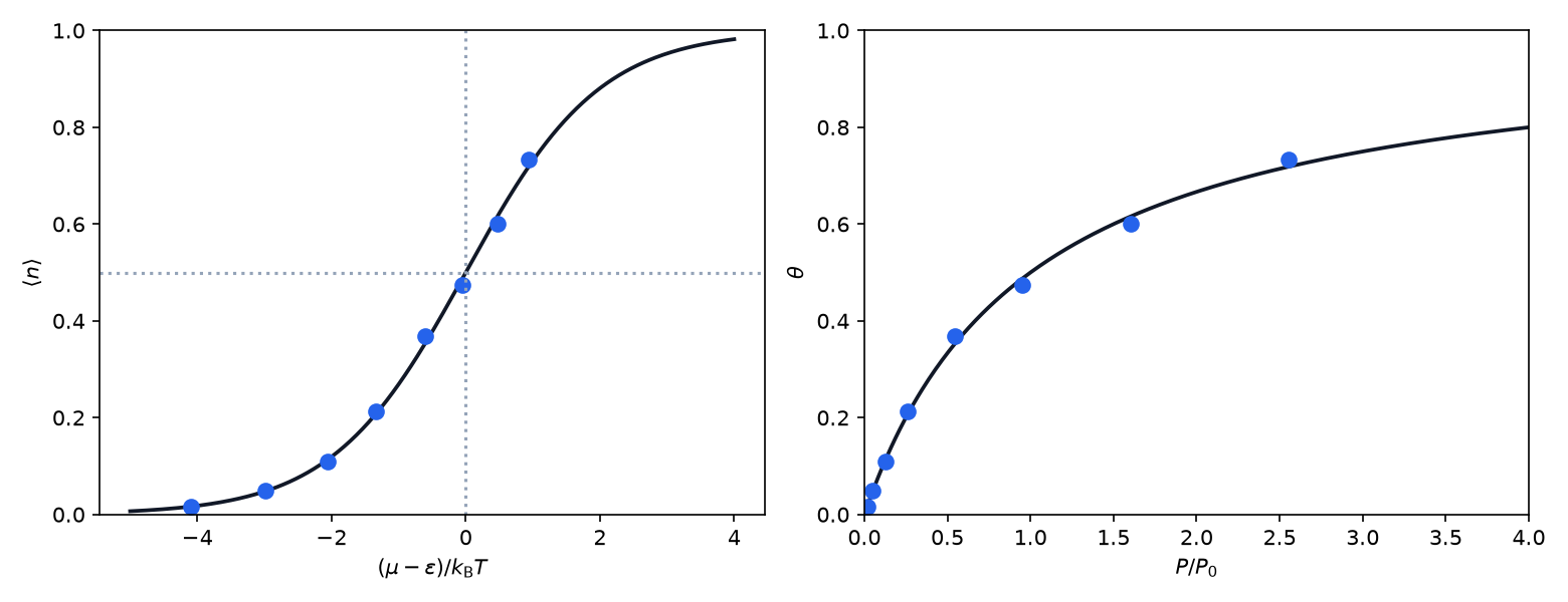
(a) Fraction of surface sites occupied against the reservoir’s chemical potential, relative to the binding energy, . The black curve is the one-site grand-canonical result ; the blue points are simulated, each the average of the second half of one run, at eight particle numbers. (b) The same points against , which for a dilute gas is its pressure in units of — the Langmuir isotherm . The reservoir here is up to full, where its density and differ by more than a tenth; that is why the axis is not the density.
| particles in total | 20 | 150 | 600 | 1000 | 2400 |
|---|---|---|---|---|---|
| common () | -7.09 | -5.05 | -3.61 | -3.05 | -2.06 |
| exact coverage | 0.0165 | 0.1140 | 0.3533 | 0.4871 | 0.7187 |
| 0.0165 | 0.1139 | 0.3532 | 0.4870 | 0.7186 | |
| simulated | 0.0165 | 0.109 | 0.369 | 0.474 | 0.734 |
The exact coverage counts every way of sharing the particles between surface and reservoir. The formula needs only one number, the chemical potential that the two share, and reproduces it to 10-4. The surface does not know how big the reservoir is, or how many particles are in it. It responds only to . The simulated coverages scatter about both by a few hundredths — two hundred sites, each full or empty, averaged over a finite run.
9. Osmosis. For sucrose in water at , with the ideal-solution model:
| concentration (mol/L) | 0.01 | 0.1 | 0.5 | 1.0 |
|---|---|---|---|---|
| van 't Hoff (MPa) | 0.0248 | 0.248 | 1.239 | 2.479 |
| (MPa) | 0.0248 | 0.248 | 1.245 | 2.502 |
| difference |
A 0.1-molar solution — of sugar in a litre of water — has an osmotic pressure of , enough to hold up a column of water tall.
The falsifying experiment for osmosis. Which way something crosses a membrane can be weighed. Dissolve the shell of a raw egg in vinegar, leaving the egg inside its own membrane, which passes water far more readily than sugar. Left overnight in pure water, it swells and gains mass. Left in concentrated sugar syrup instead, it shrivels and loses mass. If osmosis were sugar pushed through the membrane, the egg in syrup would take up sugar and swell; it does the opposite. What crosses is the water, moving toward the side where its chemical potential is lower — into the egg from pure water, out of the egg into the syrup.
10. A measurement. The laboratory generates synthetic readings of at six concentrations, with a random error on each, standing in for a class’s dialysis-tubing experiment. Fitting against the molar concentration gives a slope of , against at : van 't Hoff’s law turned around, an estimate of the gas constant from sugar water, within two standard errors.
Transfer the idea
Wherever particles — molecules, electrons, defects, photons — can move between two places or two forms, equilibrium is equal chemical potential.
Phase coexistence. Water and its vapour in a closed flask exchange molecules. They coexist when — two “boxes” that happen to be two phases of one substance. That single condition gives the boiling curve, and it is module 14’s first equation.
The Fermi–Dirac function. Step 6’s site occupation, , is the occupation of an electron state in a metal, with the electrons’ own chemical potential. Module 17 derives it for every quantum state and explains why the chemical potential of an electron gas is positive: for electrons in copper at room temperature , far outside the classical regime where .
The entropy of mixing. Module 08 promised a quantitative account of mixing and of the Gibbs paradox. Step 6’s ideal solution is that account: mixing two different species changes each one’s chemical potential by and produces the entropy ; “mixing” two samples of the same gas changes no chemical potential, and produces none.
Semiconductors. Electrons and holes in silicon are created in pairs and destroyed in pairs. Treating the reaction with the law of mass action gives , a constant fixed by temperature alone: doping that raises one carrier’s density lowers the other’s in proportion.
Defects in crystals. A vacancy is a “particle” that can be created at the surface and moved into the bulk; equal chemical potential for vacancies gives module 11’s as a mass-action result.
Living cells. A red blood cell in pure water swells and bursts; in concentrated salt water it shrivels. The osmotic pressure of blood, about 0.3 moles of dissolved particles per litre at , is — which is why intravenous fluids are made to match it.
Reverse osmosis. Seawater’s dissolved ions give it an osmotic pressure near . Push harder than that on the seawater side of a membrane, and the solvent’s chemical potential there rises above that of fresh water: water flows out of the brine. Desalination plants run at 50 to .
Looking ahead:
Module 14 applies equal chemical potential between phases, and derives the Clausius–Clapeyron equation from it.
Module 17 normalizes the grand-canonical weight over every state and every particle number, derives , and follows of quantum gases toward zero and beyond.
Module 18 asks how fast particles flow down a chemical-potential difference; this module has only said where they end up.
Worked examples
Try each one before opening its solution.
Worked example 1 — the chemical potential of air. Find and for nitrogen () at and .
Solution
. With ,
so and . Air is six million times more dilute than the quantum concentration: deeply classical.
Worked example 2 — two boxes, one offset. Box B’s floor is above box A’s; the boxes are the same size and hold 1000 particles between them, dilutely. How many end up in A?
Solution
, and with equal volumes too. So , and .
Worked example 3 — a mountain. Using constant chemical potential, find the ratio of the nitrogen density at the top of a mountain to that at sea level, for an isothermal atmosphere at .
Solution
is the same at both heights, so . The scale height is , so the ratio is . The real atmosphere is colder at altitude and the true ratio is somewhat different — the isothermal column is a model.
Worked example 4 — a site at its half-filling point. A surface site binds a molecule with , at (). What fraction of the time is it occupied when the gas has ? When ?
Solution
in the first case, so . In the second it is -1.93, and . The two answers add to one: the function is symmetric about .
Worked example 5 — a reaction. Molecules convert between forms A and B, with B higher by and equal quantum concentrations. What fraction is B? What if B’s is three times A’s — for instance, because B has three internal states of the same energy?
Solution
, so a fraction is B. With the factor three, , and B’s share rises to 0.289. Entropy — more ways of being B — partly offsets energy.
Worked example 6 — how tall a column? A bag of 0.1-molar sugar solution is closed by a membrane at the bottom of a tube and dipped in pure water at . How high does the solution rise in the tube?
Solution
. The column stops rising when its hydrostatic pressure equals , so — ignoring the dilution caused by the water that flows in, which lowers it in practice.
Check your understanding
Two boxes at the same temperature exchange particles through a small hole. When the exchange has stopped on average, which quantity is certainly the same in both boxes?
A. The chemical potential mu. B. The concentration (particles per unit volume). C. The number of particles. D. The energy per particle.
Check your answer
Correct answer: A — The chemical potential mu.
A. Right. Maximizing the total entropy over the split of the particles gives dS_1/dN_1 = dS_2/dN_2, which at a common temperature is mu_1 = mu_2. In the laboratory two boxes whose floors differ by 2 k_B T settle at densities seven to one, with equal mu.
B. This is the misconception that particles always flow from high to low concentration. Density enters only through the entropic part of mu, k_B T ln(n/n_Q); if a particle has a different energy in each box, the densities end up unequal -- by exp(-Delta u/(k_B T)) -- and stay that way.
C. Nothing favours equal numbers: two boxes of different sizes with no energy offset end with equal densities, so the larger box holds more particles.
D. Two boxes with no floors and no forces have the same energy per particle from the start, yet particles flow from the more crowded one. The chemical potential includes an entropic term that the energy per particle does not.
A system at fixed U and V has S/k_B = 1000.00 at N = 500 and S/k_B = 1004.00 at N = 502, at temperature T. Estimate its chemical potential, in units of k_B T.
Check your answer
Correct answer: -2.0 (± 0.05)
mu = -T (dS/dN) at fixed U, V. The slope is (1004.00 - 1000.00) k_B / 2 = 2 k_B per particle, so mu = -2 k_B T. If you answered +2, you dropped the minus sign in the definition: adding particles that add entropy makes mu negative.
For a pure substance, G = mu N but F is not mu N. Why?
A. G’s natural variables T and P are intensive, so by extensivity G/N depends on T and P only -- and the Euler relation gives G = U - TS + PV = mu N; F = U - TS = mu N - PV depends on V as well. B. Because mu is defined as dG/dN, while F has no derivative with respect to N. C. Because G = mu N is only true for an ideal gas. D. Because F includes the kinetic energy of the particles and G does not.
Check your answer
Correct answer: A — G’s natural variables T and P are intensive, so by extensivity G/N depends on T and P only -- and the Euler relation gives G = U - TS + PV = mu N; F = U - TS = mu N - PV depends on V as well.
A. Right. The Euler relation U = TS - PV + mu N, from extensivity alone, gives both results. G has one extensive natural variable, N, so it is N times a function of intensive variables -- and that function is mu. F has two, V and N.
B. F does have one: mu = (dF/dN) at fixed T and V, too. Both derivatives give the same mu; what differs is whether the potential equals N times its derivative, and that depends on which other variables are extensive.
C. It holds for any one-component system whose entropy is extensive. The ideal gas is just the case where the laboratory checks it numerically.
D. Both contain U. They differ by PV, which is exactly the term that makes F = mu N - PV.
Box 1 holds a gas at density 2 n_0 with mu_1 = -6 k_B T; box 2 holds a gas of the same species at density n_0 with mu_2 = -4 k_B T. The temperatures are equal. A hole is opened between them. What happens?
A. Particles flow from box 2 into box 1, the denser box, because mu_2 > mu_1. B. Particles flow from box 1 into box 2, because box 1 is denser. C. Particles flow until the energy per particle is the same in both boxes, then stop. D. Nothing flows, because the temperatures are equal.
Check your answer
Correct answer: A — Particles flow from box 2 into box 1, the denser box, because mu_2 > mu_1.
A. Right. dS_tot = (mu_2 - mu_1) dN_1 / T > 0 for dN_1 > 0: particles flow from high mu to low, whatever the densities. Box 1 must have a lower floor -- an attractive wall, a lower height -- that makes its mu lower despite the crowding.
B. This is the concentration rule, and it fails whenever the boxes differ in anything but density. The chemical potentials rank the other way, and they decide.
C. This is the misconception that the chemical potential is just the energy per particle. Equal energies per particle do not stop the flow: in the laboratory, two boxes with no floors at all -- the same energy per particle from the start -- still exchange particles until their densities match, because mu has an entropic part. Flow stops at equal mu.
D. Equal temperatures stop the flow of energy, not of particles. Particle exchange needs equal mu as well.
In an isothermal atmosphere of nitrogen at 288 K the scale height k_B T/(m g) is 8.72 km. Using constant mu, what is the ratio of the density at 3.0 km to the density at sea level?
Check your answer
Correct answer: 0.709 (± 0.005)
k_B T ln n(z) + m g z is the same at both heights, so n(z)/n(0) = exp(-z/H) = exp(-3.0/8.72) = 0.709. If you answered 0.656, you used 7.1 km, a scale height for a colder or heavier gas, since H = k_B T/(m g); if 0.344, you gave z/H itself rather than the exponential.
The grand-canonical weight P(s) ~ exp(-(E_s - mu N_s)/(k_B T)) is a theorem. Which hypotheses does it need?
A. A reservoir large enough that its temperature and chemical potential stay fixed when it gives up energy and particles, and coupling weak enough that energies and particle numbers add. B. Every state (E_s, N_s) of the system must be equally probable. C. The system must be an ideal gas. D. The system must hold many particles, so that Stirling’s approximation applies to it.
Check your answer
Correct answer: A — A reservoir large enough that its temperature and chemical potential stay fixed when it gives up energy and particles, and coupling weak enough that energies and particle numbers add.
A. Right. The derivation expands the reservoir’s entropy to first order in the energy and particles it gives up; the neglected second-order terms are small only for a large reservoir. Weak coupling is what makes E_total = E_s + E_R.
B. The opposite: states are weighted unequally, by exp(-(E_s - mu N_s)/(k_B T)). Equal probability belongs to the isolated system plus reservoir as a whole, not to the small system -- the same trap as reading the canonical ensemble as equal probability.
C. Nothing about the system is assumed. The module applies the weight to a single adsorption site, which is not a gas at all.
D. Stirling is needed for the reservoir’s smooth entropy, not for the system. The weight holds for a system of one site holding zero or one particle.
An adsorption site with binding energy epsilon is in contact with a gas at chemical potential mu, where (epsilon - mu)/(k_B T) = 1.5. What is its mean occupation?
Check your answer
Correct answer: 0.182 (± 0.003)
= 1/(exp((epsilon - mu)/(k_B T)) + 1) = 1/(exp(1.5) + 1) = 1/(4.48 + 1) = 0.182. If you answered 0.223, you gave exp(-1.5), the Boltzmann ratio without the +1 of single occupancy; if 0.818, you swapped the sign of epsilon - mu.
Molecules convert between forms A and B. Form B lies 1.0 k_B T above form A and has twice A’s quantum concentration (two internal states of equal energy). What is n_B/n_A at equilibrium?
Check your answer
Correct answer: 0.736 (± 0.01)
mu_A = mu_B with mu_X = k_B T ln(n_X/n_Q,X) + epsilon_X gives n_B/n_A = (n_Q,B/n_Q,A) exp(-Delta epsilon/(k_B T)) = 2 exp(-1) = 0.736. If you answered 0.368, you left out the factor of two -- the extra ways of being B.
A dialysis bag holding 0.2 mol/L sucrose solution is put in pure water at 298 K. The bag’s wall passes water but not sucrose. What happens, and how large is the osmotic pressure?
A. Water flows into the bag, which swells; the osmotic pressure is about n_s k_B T = 5 bar. B. Sucrose flows out of the bag until the concentrations are equal; the pressure is about 5 bar. C. Water flows out of the bag, which shrinks, because the solution is denser. D. Nothing happens, because no pump is present.
Check your answer
Correct answer: A — Water flows into the bag, which swells; the osmotic pressure is about n_s k_B T = 5 bar.
A. Right. Sucrose lowers the water’s chemical potential inside the bag by about -k_B T ln(1 - x), so water flows in, toward the lower mu. It would stop only if the inside were at a higher pressure by Pi = n_s k_B T = 0.2 x 1000 x N_A x k_B x 298 = 5.0 x 10^5 Pa.
B. This is the misconception that osmosis is solute pushed through the membrane. The sucrose cannot cross at all. It is the water that moves, down its own chemical-potential difference.
C. The solution’s water has the lower chemical potential, so water flows in, not out. A bag of pure water in a sugar bath would shrink.
D. No pump is needed. Water flows down its chemical-potential difference as particles in the two-box simulation flow down theirs.
In three or four sentences: why is the chemical potential of a classical ideal gas negative, and what would it signal if a gas’s mu approached zero?
Check your answer
For the ideal gas mu = k_B T ln(n/n_Q), with n_Q the quantum concentration, one particle per thermal wavelength cubed. A gas is classical exactly when n is far below n_Q -- air at room conditions is six million times more dilute -- so the logarithm is negative. Physically, adding a particle to a dilute gas adds entropy (it has a great deal of room), and mu = -T dS/dN is negative whenever dS/dN is positive. mu approaching zero means n approaching n_Q: the thermal wavelengths overlap, the classical counting behind Sackur-Tetrode fails, and quantum statistics (module 17) take over. A strong answer names both the entropic reason and the n_Q criterion.
Exam-style problems for this module — the ones worth doing with a pen — are collected in the problem set.
Explain it in your own words
Answer in a few sentences each.
A chemist friend says that particles can only move from high to low concentration unless something pumps them. Explain why two connected boxes can hold particles at a seven-to-one density ratio with no pump at all.
Why is the chemical potential of a classical ideal gas negative? What would it signal if a gas’s approached zero?
What does have to do with ? Why is but ?
In osmosis, what flows, what does not, and what is the osmotic pressure the price of?
Advanced: fugacity, activity, and why mu is not a free variable
Fugacity. Step 4’s ideal gas has , or, per mole and in terms of the pressure, , with a chosen reference pressure. A real gas does not obey this. Rather than give up the convenient logarithm, chemical engineers keep it and define a corrected pressure , the fugacity, so that holds exactly. For a dilute gas . Fugacity is therefore bookkeeping for in the units of a pressure, and equal chemical potentials become equal fugacities — which is how phase equilibria are tabulated in practice.
Activity. The same device applied to a solution: the activity of a component is defined by . In step 6’s ideal solution the solvent’s activity is its fraction, . Real solutions have activity coefficients that differ from one, and measuring them — often by osmotic pressure — is how the departure from the ideal model is quantified. The sucrose example at the end of the verification is exactly such a departure.
Gibbs–Duhem, re-read. Module 09 derived
from extensivity. For one component it says that , and cannot be varied independently: fix the temperature and the pressure, and the chemical potential is fixed too, with per particle. That is step 3’s again, now with its derivatives: is the step the osmotic derivation used. For a mixture of components the relation leaves independent intensive variables, and counting them across coexisting phases gives module 14’s phase rule.