Quantum statistics — Bose–Einstein and Fermi–Dirac gases
Quantum statistics: Bose–Einstein and Fermi–Dirac gases
The puzzle: identical particles, opposite habits
The copper in a phone charger is a box full of gas. Each copper atom gives up one electron to the metal as a whole, and those conduction electrons — of them in every cubic metre — move through the crystal much as molecules move through a container. Module 04 knows what to do with a gas: give every particle of kinetic energy, and the gas has a heat capacity of per mole. A mole of copper atoms therefore ought to need for its lattice (module 16’s Dulong–Petit value) plus another for its electrons: half as much again.
It does not. Measured at room temperature, metals sit at Dulong–Petit, and the electrons’ share of the heat capacity is less than one part in a hundred. A gas that should dominate the heat capacity of every metal barely registers. Where does its heat capacity go?
The second gas goes the other way. Cool liquid helium-4 below and it turns into a superfluid: it flows without friction through pores so fine that the ordinary liquid is held back, and creeps up the walls of its container. In 1995 a cloud of rubidium-87 atoms was cooled to a few hundred billionths of a kelvin, and a large fraction of the atoms — all identical — was found in one and the same quantum state, the lowest one the trap allowed.
The answer adds exactly one thing to the course: a rule for how many identical particles may share a state. No wave functions, no operators. Everything else is counting, and module 13’s chemical potential.
Predict before you calculate
Commit to an answer for each of these before reading on. Write them down.
A gas of electrons is cooled toward absolute zero at fixed density. Equipartition says the mean kinetic energy per electron, , goes to zero. Does it?
Three single-particle states share the same value of : one in a classical gas, one in a gas of bosons, one in a gas of fermions. Rank the mean number of particles each holds.
Are the conduction electrons in copper at room temperature a classical gas or a quantum one? And is that decided by the temperature, or by something else?
Below the condensation temperature a large fraction of a Bose gas sits in the lowest state, which has no kinetic energy. Does the gas still push on its walls? If it does, how does the pressure depend on how much gas there is?
Explore the model
The laboratory has four explorers. The first draws the mean occupation of a state against its energy for bosons, fermions and classical particles, with sliders for the temperature and the chemical potential, and a logarithmic view. The second follows a Bose gas through condensation, both for the ideal infinite gas and for a box of a thousand to a hundred thousand atoms counted level by level. The third fills a Fermi sea and shows which electrons can still take up heat. The fourth tracks the chemical potential of all three gases at one density as the temperature falls. Then the laboratory runs the experiments this module is built on: the occupations rebuilt from explicit sums, the states of a box counted one by one, the chemical potential solved for at fixed density, module 16’s Planck spectrum rebuilt from a boson occupation, and a measurement of the conduction electrons of silver.
Three gases at the same density and temperature: bosons (blue), classical particles (black, dashed) and fermions (red), each with its own chemical potential, as the gas is heated at fixed density so that falls from 2.5 to 0.001. Left: the mean occupation of a state against its energy, divided by so that the classical curve, , stays put. In the dense gas the bosons crowd into the lowest states and the fermions, barred from crowding, are pushed out to higher energies; as the gas thins, both fall onto the classical line. Right: for each gas against , with a marker at the current value. The three agree when the gas is dilute; above the fermions’ climbs above the classical one and the bosons’ flattens at zero, which it reaches at (dotted).
Run the laboratory now, then come back. Four things are worth doing before you read on:
In the occupation explorer, set well below zero and switch to the logarithmic view. Then raise toward zero. Where do the three curves part company?
Try to push the bosons’ above the lowest energy. What does the explorer do, and why?
In the condensation explorer, compare a box of a thousand atoms with one of a hundred thousand near .
In the Fermi-sea explorer, lower from 1 to 0.01 and watch which part of the sea changes.
Derive the result
System and boundary. An ideal gas of identical particles of mass in a cubic box of side and volume with rigid walls, in contact with a heat bath at temperature . Each single-particle state is treated as a subsystem that exchanges energy and particles with the rest of the gas, which acts as its reservoir.
Independent variables. The temperature , the volume and the number of particles — equivalently the density . The chemical potential is not an independent variable here: it is whatever value makes the gas hold particles.
Sign convention. The course convention, , holds. It is exercised in step 7: squeezing a Fermi gas at absolute zero takes work, when , and with all of it becomes energy of the gas.
Units. SI throughout, with , and written explicitly. Energies are in joules; the electronvolt, , appears only as a convenience in quoted numbers.
Route. Nine steps. State the rule for identical particles and see what it does to counting; put one state in contact with a reservoir and find its mean occupation, for bosons and for fermions; take the dilute limit, which is classical physics; count the states of a box; fix the number of particles, which fixes ; and then follow the consequences — condensation for bosons, the Fermi sea and its pressure for fermions, the heat capacity of a metal, and, as a corollary, module 16’s photons.
Step 1: identical particles
Module 08 counted microstates of coins and module 12 of molecules, and both times a question was left hanging: when two particles are of the same kind, is swapping them a new microstate? Module 12 answered “no” by dividing by , and justified it only for a gas so thin that no two particles ever compete for one state. Quantum mechanics answers the question exactly, and the answer is the only quantum input this module needs.
Count the states of two particles shared between two single-particle states, and .
| classical (labelled) | bosons | fermions | |
|---|---|---|---|
| both in | 1 | 1 | 0 |
| one in each | 2 | 1 | 1 |
| both in | 1 | 1 | 0 |
| total | 4 | 3 | 1 |
Classical particles carry labels, so “particle 1 in , particle 2 in ” and the reverse are two microstates. For identical particles they are one. The exclusion rule then removes the states with two fermions together. If every microstate is equally likely, as module 08 assumed, the chance of finding the two particles in the same state is classically, for bosons and 0 for fermions. Bosons bunch and fermions avoid one another — and no force is involved. It is counting.
The same counting explains module 12’s . Spread particles over single-particle states. Classical particles have arrangements, and module 12’s corrected count is . Bosons have and fermions . When the states far outnumber the particles, , both quantum counts approach : three particles in a hundred states give 1.03 and 0.97 times it, in a thousand states 1.003 and 0.997. Dividing by was quantum statistics in the limit where it does not matter which kind it is.
Step 2: one state in contact with a reservoir
Module 13 put a single adsorption site in contact with a gas and weighted each of its states by , where is the number of particles the site holds. Apply the same argument to one single-particle state of energy : holding particles, it has energy , and its weight is .
For bosons runs over and the sum is module 12’s geometric series. Write :
which converges only if . The mean occupation is the same derivative that gave module 12 its mean energy, .
As rises toward , the lowest state’s occupation grows without limit. The bound is not a technicality: step 6 is what happens when a gas presses against it.
For fermions is 0 or 1, and the sum has two terms:
This is module 13’s site occupation, unchanged: an electron state is a site that holds at most one particle. Module 13 said the function would come back under this name, and here it is.
The mean is not the whole story. The occupation of a state fluctuates, and its variance is for bosons, for fermions, and for classical particles. Bosons fluctuate more than classical particles — the bunching of the counting table, seen in a single state — and fermions less. The laboratory draws occupations at random from each distribution and checks all three.
Step 3: the classical corner
Both distributions differ from each other only in the sign of the 1 in the denominator. When is large, that 1 does not matter.
When the three agree to : and . The condition holds for every state at once when lies far below the lowest energy — when every state is so sparsely occupied that no two particles ever compete for one, and whether they could share it never comes up. That is classical physics. Step 5 turns “ far below zero” into a statement about density and temperature.
Step 4: counting the states of a box
The single-particle states of a cube with hard walls are standing waves, exactly as module 16’s cavity modes were. Each has wave vector
and, for a particle of mass , kinetic energy . Counting the states with energy below is counting integer points inside an octant of a sphere of radius , one point per unit volume when the radius is large. With spin states for each wave,
The count is module 16’s, with one change: there, for a photon, and the density of modes grew as ; here , and it grows as . The approximation of counting volume instead of points misses the states on the octant’s faces, a relative error of about , and the laboratory measures it. It is negligible: for helium in a box the lowest level spacing is in temperature units, and at the states that matter have of about ten million.
Step 5: holding the number of particles fixed
Multiply the number of states by their mean occupation and integrate:
For a given , and this is one equation for one unknown, . Substituting collects the constants into one length, module 12’s thermal wavelength.
With these, the integral over states becomes one line:
For classical particles the integral can be done by hand: , and
This is module 13’s , with . Module 13 named the quantum concentration and promised that this module would derive it: here it is, the density at which the gas has one particle per spin state in each cube of side .
For bosons and fermions there is no closed form, and is found numerically: given , find the at which . The laboratory does it by bisection, and its result, which knows nothing of module 13, reproduces module 13’s classical formula to sixteen digits in the dilute limit.
The criterion involves the density, the mass and the temperature together. Air at room temperature has , and helium gas at and one atmosphere : profoundly classical. Liquid helium at has 4.5. The conduction electrons in copper at room temperature have 6800: an electron is 7300 times lighter than a helium atom, so its thermal wavelength at is , nineteen times the spacing between electrons.
Which way does move as a gas is cooled at fixed density? grows as , so must grow, and must climb. How far it can climb depends on the statistics:
| (with ) | 0.01 | 0.1 | 1 | 2.612 | 10 |
|---|---|---|---|---|---|
| classical, | -4.605 | -2.303 | 0 | 0.960 | 2.303 |
| bosons, | -4.609 | -2.338 | -0.359 | 0 | 0 |
| fermions, | -4.602 | -2.267 | 0.349 | 1.852 | 5.456 |
The classical formula takes above zero once ; it then predicts more than one particle in the lowest states, which is the classical theory leaving the domain it was derived in. The bosons’ climbs to zero — the lowest energy — and stops there, at . The fermions’ climbs without limit; as , step 7 shows, tends to a fixed positive energy, .
Two more integrals give the energy and the pressure. The energy is , and the pressure needs no new calculation at all.
Module 04 derived it from the momentum carried to the walls: , and is twice the kinetic energy. Nothing in that argument asks how many particles share a state. For a classical gas and it is the ideal gas law.
Step 6: Bose–Einstein condensation
The bosons’ stops at zero, and stops with it. The largest value the occupation integral can take is
a pure number — it is , where is the Riemann zeta function; this module quotes the value and the laboratory computes it by quadrature.
Below the excited states are full and cannot take the rest. The particles have one place left to go: the ground state, which the integral never counted — its density of states gives it zero weight at , although it is a perfectly good state that can hold any number of bosons. The ground state takes the overflow.
An ideal Bose gas cooled at fixed density from to , pausing at . Left: the share of the particles in the ground state (dark blue) and in all the excited states together (light blue). Middle: how the excited particles are spread over energy, in units of ; the area under the curve is their share. At the curve rises sharply toward zero energy, but its area is still all the particles; below it shrinks, as , and the ground state holds the rest. Right: the condensate fraction against — the ideal (black, with the moving dot), and the exact result for a box of 103 atoms (grey, dashed) and of 105 atoms (amber, dashed), computed level by level. The finite boxes condense earlier and more gradually, and approach the ideal curve as they grow.
Condensation is a statement about occupation, not about motion. Below the excited particles are exactly as many as the excited states can hold at that temperature, and they move and collide with the walls as before. Only they carry energy, so by step 5
where 1.341 is . This pressure is not zero, and it does not depend on the density at all: add atoms to a condensed gas at fixed temperature and they join the condensate, which carries no momentum to the walls. At the pressure is of the classical . The heat capacity, for a hot gas, rises as the gas cools toward , peaks there at with a sharp corner, and falls below it as .
Step 7: the degenerate Fermi gas
Fermions cannot condense: each state takes one. Cool a Fermi gas to and the occupation becomes a step — every state below is full, every state above it empty. The particles fill the box’s states from the bottom, per standing wave, and the energy of the last one filled is the Fermi energy . Step 4’s count gives it at once: .
The energy follows from : the mean of weighted by over 0 to is . The pressure is worth deriving a second way, with the course’s sign convention. Every level of the box is proportional to , so the energy of the filled sea is . At absolute zero the sea stays in its ground state as it is squeezed slowly — the occupations cannot change — so no heat flows, , and :
This is the degeneracy pressure. Squeezing the sea raises every level, and the work done on it is stored as the energy of the raised levels.
For copper, with one conduction electron per atom, , and with and the electron’s mass:
, so ;
the fastest electrons move at , the Fermi velocity;
the mean kinetic energy is — a classical gas would need to have it;
the degeneracy pressure is , atmospheres, against for a classical gas of the same density at room temperature — more than a hundred times larger.
All of this is at absolute zero, and none of it involves a force: the model’s Ignored line lists every interaction between the electrons. The pressure is kinetic energy, delivered to the walls as in module 04. What holds the electrons in a real metal is the attraction of the positive ions, which the model’s rigid walls stand in for.
A Fermi gas cooled from to at fixed density. Left: the density of states (grey) and the occupied part of it, (blue), against ; the dashed line is the Fermi energy and the amber triangle the chemical potential. The amber band, wide, centred on , marks the electrons that a temperature can still move: below it every state is full and above it every state is empty. As the gas cools, the edge hardens into a step at , climbs to , and the band narrows, while the bulk of the sea does not change. Right: the heat capacity per particle, , on logarithmic axes, against (blue, with the moving dot): it is the classical when hot (dotted) and follows the straight line (red, dashed) when cold.
Step 8: why a metal’s electrons store almost no heat
Heating a Fermi gas by offers every electron an extra energy of order . An electron deep in the sea cannot accept it: every state within of its own is already taken. Only the electrons within about of the top of the sea have empty states above them to move into, and they are a fraction of order of the whole.
For copper at room temperature, : the electrons’ heat capacity is of the classical , and of the lattice’s . That is the puzzle’s missing heat capacity. It was never missing: it was frozen out, not by quantization of the energy, as in module 16, but by exclusion.
At low temperature the lattice’s contribution falls as (module 16) and the electrons’ only as , so in every metal there is a temperature below which the electrons dominate. Per mole of atoms with conduction electrons each,
with module 16’s Debye coefficient. Plotting against gives a straight line whose intercept measures the electrons and whose slope measures the lattice. The verification below does this with real data.
Step 9: photons, the bosons with μ = 0
Module 16 derived Planck’s law from the oscillator, mode by mode. The same result follows from this module in one line. Photons are bosons, so a mode of frequency holds on average of them. But the walls absorb and emit photons freely, so their number is not conserved: there is no to hold fixed, and no step 5. As module 16 showed, the free energy is then lowest at .
A photon gas cannot condense, for the same reason it has . Condensation needed a fixed number of particles pressing against its bound; photons that do not fit are simply absorbed by the walls.
Verify computationally
Every number below comes from thermolab.quantum, which evaluates the occupation integrals by
quadrature and solves for by bisection, with no special functions. Nothing in this module is
random except two checks that sample on purpose. The laboratory repeats each experiment.
1. The occupations, rebuilt from explicit sums. Summing a state’s grand-canonical weights term by term — from 0 to 4000 for bosons, with for classical particles, two terms for fermions — reproduces the closed forms of step 2 to at , 0.5, 2 and 10, and the variances , and to the same precision. Drawing occupations at random at gives a boson mean of 1.539 and variance 3.89, against 1.541 and 3.92.
2. Counting, one state at a time. Listing every arrangement of two particles in two states gives 4, 3 and 1. Listing the states of a cube one by one and comparing with step 4’s smooth count: the explicit count falls short by at , at 80 and at 320. The shortfall times settles at : the missing states on the octant’s faces, and nothing else.
3. The classical corner. Across from 100 to the boson and fermion occupations never differ from the classical one by more than and , and below 100 they are ordered everywhere.
4. The density fixes μ.
The classical solver, which inverts the quadrature and knows nothing of module 13, reproduces module 13’s to . And particle number is conserved in the code: for each statistics, at temperatures from to , integrating afresh at the solved — on a different grid, with Simpson’s rule — returns the density that was put in, to 10-9.
5. Condensation in a real box. The ideal condensate fraction is a limit. The laboratory also computes it exactly, for spinless bosons in a hard-walled cube, by summing over the box’s levels one by one, with no density of states and no integral. At , where the ideal fraction is 0.646:
| atoms | 103 | 104 | 105 | 106 |
|---|---|---|---|---|
| at | 0.782 | 0.732 | 0.698 | 0.676 |
| at | 0.323 | 0.198 | 0.116 | 0.066 |
| fitted exponent of | 1.68 | 1.61 | 1.56 | 1.54 |
A finite box condenses early, because its hard walls remove the states on the octant’s faces and the excited states fill sooner. The excess shrinks slowly — the fraction at exceeds the ideal by to within across the whole table, a surface effect — and the fitted exponent drifts down toward . The ideal theory is the large- limit of the real count, approached at the rate a surface correction allows.
6. The degenerate Fermi gas. For electrons at copper’s density, the numerically solved at is to within 10-6, and the energy per particle and the pressure exceed and by four parts in a million — the size of the correction the Sommerfeld expansion predicts. The heat capacity, obtained from the occupation integrals, is to 1 part in 104 at , still of it at , and falls below the line from about , levelling off at above .
7. Against reality: the electrons in silver. Module 16 fitted silver’s measured heat capacity, tabulated by NIST (Smith and Fickett, 1995), below to , and set the electrons’ term aside. Here it is the measurement.
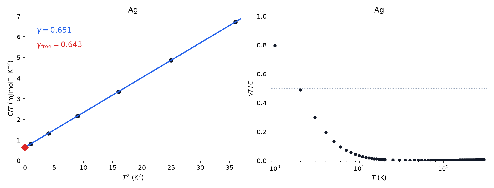
Left: silver’s molar heat capacity below , as against (black points), with the least-squares line (blue). Its intercept is the electrons’ coefficient ; the red diamond on the axis is the free-electron prediction, 0.643, computed from silver’s density alone. The slope is the lattice’s Debye term. Right: the electrons’ share of the measured heat capacity, , from 1 to : at , about half at , and at room temperature.
The measurement. The fit gives (statistical; ending the window at instead of 6 gives 0.649, the systematic scale of the number).
The prediction. Silver has one conduction electron per atom; its density, , and molar mass, , give , and , and so . The measurement is 1.01 times the prediction.
The share. The electrons carry of silver’s heat capacity at and half of it at , where ; at room temperature they carry — the puzzle’s “missing” heat capacity, measured.
Silver is the best case. A metal’s electrons feel its lattice, and the ratio of measured to free-electron , called the thermal effective mass, records how much. With measured values from Kittel’s table (8th edition, p. 139) and free-electron values computed here from each metal’s room-temperature density:
| metal | measured | free-electron | ratio | |
|---|---|---|---|---|
| Ag | 1 | 0.646 | 0.643 | 1.00 |
| Au | 1 | 0.729 | 0.640 | 1.14 |
| Cu | 1 | 0.695 | 0.502 | 1.38 |
| Al | 3 | 1.35 | 0.910 | 1.48 |
(in ). The free-electron gas gets the size and the linearity right for all four and the coefficient right to within a factor of 1.5; the rest is band structure, which this model ignores by name.
8. Against reality: liquid helium-4. Is the superfluid transition of helium a Bose–Einstein condensation? At the density of liquid helium at its transition, (Donnelly and Barenghi, 1998), step 6 gives
against the measured transition, the lambda point, at . The ideal gas misses by . It misses in a telling way: it is the right order of magnitude, from nothing but the mass and the density, and liquid helium is the least ideal gas imaginable. Its atoms sit apart, closer than their thermal wavelength of and close enough to repel strongly. London proposed the connection in 1938 from this very estimate; the modern view is that the superfluid is a condensate, strongly modified by interactions — neutron scattering finds less than a tenth of the atoms in the zero-momentum state even at absolute zero, where the ideal gas would put them all. The ideal model locates the phenomenon; it does not describe the liquid. That is its Failure modes line, measured.
The falsifying experiments. Each misconception this module confronts has a measurement above that it cannot survive. “Quantum effects matter only when it is cold”: copper’s electrons at room temperature have and , and silver’s measured , set by the Fermi temperature of , confirms it — degeneracy is set by , not by alone. “Condensation is the atoms stopping”: below the excited states hold particles and the pressure is , nonzero and independent of how many atoms are in the condensate (item 5 and step 6). “A Pauli force pushes fermions apart”: the degeneracy pressure of item 6, for copper, comes out of a model whose Ignored line lists every interaction; it is counting and kinetic energy, not a force.
Transfer the idea
One rule — how many identical particles may share a state — split the ideal gas into two gases with nothing classical about them. It reaches back through the course and out into the world.
Back to modules 08 and 12. The Gibbs , which module 12 justified for a dilute gas only, is the common dilute limit of the Bose and Fermi counts (step 1).
Back to module 13. The quantum concentration is derived: , and module 13’s is the dilute limit of . Module 13’s one-site argument, applied to every standing wave, is this module’s step 2, and its Langmuir site occupation is the Fermi–Dirac function.
Back to module 16. Planck’s law is the Bose–Einstein distribution at (step 9), and the that module 16 subtracted from silver’s heat capacity is the Fermi sea’s (step 8). A metal at low temperature is both modules at once: .
Back to module 04. is module 04’s momentum-flux pressure, for any statistics. Degeneracy pressure is delivered to the walls exactly as the pressure of air is.
Forward to module 18. Transport in a metal is carried by electrons at the Fermi velocity, in copper, not at the thermal speed of a classical gas: the only electrons that can be scattered into a new state are those at the top of the sea.
Semiconductors. The conduction electrons of pure silicon at room temperature number about 1016 per cubic metre, a ten-trillionth of copper’s. Their is tiny, and they obey Maxwell–Boltzmann statistics. The same particles are quantum in one material and classical in another: density decides.
Ultracold atoms. The first gaseous condensates were made in 1995, of rubidium-87 at about 170 billionths of a kelvin (Cornell and Wieman, Boulder) and of sodium (Ketterle, MIT), work recognized by the 2001 Nobel Prize. Those atoms were held in a magnetic trap, roughly a harmonic bowl rather than a box; there the density of states grows as , not , and the condensate fraction as — the problem set derives it. Since 2013 atoms have also been condensed in uniform, box-shaped traps (Gaunt and colleagues, Cambridge), the geometry of this module.
Helium-3. The lighter isotope of helium is a fermion. It does not condense at ; it becomes a superfluid only within a few thousandths of a kelvin of absolute zero, when its atoms pair up into bosons. The two isotopes of one element are this module’s two gases.
Stars. A white dwarf — the core a sun-like star leaves behind — is held up against its own gravity by the degeneracy pressure of its electrons; a neutron star by that of its neutrons. The advanced section estimates a white dwarf’s size.
Looking ahead:
Module 18 turns from equilibrium to the fluctuations around it and the transport they drive, and uses this module’s Fermi velocity for the electrons of a metal.
Worked examples
Try each one before opening its solution.
Worked example 1 — three particles, three states. Three particles share three single-particle states. How many microstates are there for classical particles, bosons and fermions? If every microstate is equally likely, how probable is it that all three particles are in the same state?
Solution
Classical: . Bosons: . Fermions: . All three in the same state: 3 microstates out of 27 classically (), 3 out of 10 for bosons (), and none for fermions. Bosons are almost three times as likely to be found piled up as classical particles, with no force between them.
Worked example 2 — the three occupations, side by side. A state lies one above the chemical potential. What is its mean occupation under each statistics? And at ten ?
Solution
At : , , — very different. At : , and to four figures; they differ in the fifth, by of themselves.
Worked example 3 — copper’s Fermi sea. Copper has density , molar mass and one conduction electron per atom. Find , , and the degeneracy pressure.
Solution
. , and , so and . .
Worked example 4 — the electrons’ share at room temperature. Using example 3, find copper’s electronic heat capacity per mole at and compare it with Dulong–Petit and with what a classical electron gas would contribute.
Solution
. Dulong–Petit is , so the electrons add . A classical electron gas would add , half of Dulong–Petit again — eighty-three times more than is there.
Worked example 5 — a condensate of sodium. A uniform gas of sodium-23 atoms (mass , ) has density . Find , and the fraction of the atoms in the condensate at half that temperature.
Solution
. With and , and . At , .
Worked example 6 — the classical criterion. Compute for helium gas at and one atmosphere, and for helium gas at its boiling point, , at one atmosphere. Is either quantum?
Solution
with : at and at . : and . So and 0.135. The first is deeply classical; the second is within an order of magnitude of degeneracy, and the liquid, about eleven times denser, crosses it.
Check your understanding
Two particles share two single-particle states, a and b. How many distinct two-particle states are there if the particles are classical (labelled), identical bosons, or identical fermions?
A. 4, 3 and 1 -- labelled particles can be swapped to make a new state; identical ones cannot, and fermions may not share. B. 4 in every case -- each particle still chooses one of two states. C. 3, 3 and 1 -- swapping never makes a new state, and fermions may not share. D. 4, 2 and 2 -- bosons must share a state and fermions must not.
Check your answer
Correct answer: A — 4, 3 and 1 -- labelled particles can be swapped to make a new state; identical ones cannot, and fermions may not share.
A. Right. Classically: both in a, both in b, and “1 in a, 2 in b” plus its swap -- 4. Identical bosons: both in a, both in b, one in each -- 3, because a swap of identical particles is the same state. Identical fermions: only one in each -- 1. With equal weights, the chance of finding both in one state is 1/2, 2/3 and 0: bosons bunch and fermions avoid each other, with no force involved.
B. That counts identical particles as if they carried labels. The symmetry postulate says a state of identical particles is fixed entirely by its occupation numbers, so “1 in a, 2 in b” and its swap are one state, not two. Counting by labels is classical physics.
C. For identical particles that is right, but classical particles are labelled: “particle 1 in a, particle 2 in b” and the reverse are distinct microstates, so classical counting gives 4. That difference is exactly what module 12’s division by N! was patching.
D. Bosons are allowed to share a state, not required to: one in each state is a perfectly good boson state. Fermions forbid only double occupation, which leaves the single state with one fermion in each.
In a gas of bosons the chemical potential must lie below the energy eps_0 of the lowest single-particle state. Why?
A. The lowest state’s grand sum, the sum over n of exp(-n (eps_0 - mu)/(k_B T)), converges only if mu < eps_0; as mu approaches eps_0 its mean occupation grows without limit. B. Because the chemical potential of every gas is negative. C. Because the Pauli principle forbids two bosons in the lowest state. D. Because a reservoir cannot supply particles with less energy than eps_0.
Check your answer
Correct answer: A — The lowest state’s grand sum, the sum over n of exp(-n (eps_0 - mu)/(k_B T)), converges only if mu < eps_0; as mu approaches eps_0 its mean occupation grows without limit.
A. Right. Bosons may pile up without limit, so a state’s weights form a geometric series, which converges only if each term is smaller than the last: exp(-(eps - mu)/(k_B T)) < 1, i.e. mu < eps, for every state and so for the lowest. At mu = eps_0 the lowest state would hold infinitely many particles -- which is what Bose-Einstein condensation pushes against.
B. It is not. A classical gas has mu = k_B T ln(n lambda^3), negative only when the gas is dilute, and a degenerate Fermi gas has mu close to eps_F, several electronvolts above the bottom of the box in a metal. The bound is specific to bosons.
C. The exclusion principle applies to fermions, not bosons, and the Fermi-Dirac occupation needs no bound on mu at all, because each state holds at most one particle whatever mu is.
D. The reservoir supplies particles at whatever energy the states have. The bound comes from the sum over how many particles one state can hold, not from which energies are on offer.
A single-particle state lies 2 k_B T above the chemical potential. What is its mean occupation in a gas of bosons? (Give three decimal places.)
Check your answer
Correct answer: 0.157 (± 0.002)
n_BE = 1/(e^2 - 1) = 1/6.389 = 0.157. For comparison n_MB = e^-2 = 0.135 and n_FD = 1/(e^2 + 1) = 0.119: at the same (eps - mu)/(k_B T) the order is always BE > MB > FD, because e^x - 1 < e^x < e^x + 1. At 2 k_B T they still differ by tens of percent; at (eps - mu) = 4.6 k_B T (e^x = 100) they agree within 1%.
Copper has 8.5e28 conduction electrons per cubic metre. At 300 K, roughly what is the degeneracy parameter n lambda^3 of this electron gas, and is it classical or quantum?
A. About 7000 -- deeply quantum. An electron’s thermal wavelength at 300 K is about 4 nm, nineteen times the spacing between electrons. B. About 1e-5 -- at room temperature everything is classical; quantum statistics matter only near absolute zero. C. About 1 -- borderline; room temperature sits right at the crossover. D. It cannot be decided -- the electrons’ temperature is far above 300 K, because they move at 1.6e6 m/s.
Check your answer
Correct answer: A — About 7000 -- deeply quantum. An electron’s thermal wavelength at 300 K is about 4 nm, nineteen times the spacing between electrons.
A. Right. lambda = h/sqrt(2 pi m k_B T) = 4.3 nm for the electron’s tiny mass, and n lambda^3 = 8.5e28 x (4.3e-9)^3 = 6800. Equivalently T/T_F = 300/81 700 = 0.004. What decides is n lambda^3 -- density and mass as well as temperature: helium gas at the same temperature and atmospheric pressure has n lambda^3 = 4e-6.
B. This is the misconception that quantum effects need cold. Degeneracy is set by n lambda^3, not by T alone. Helium gas at 300 K has n lambda^3 = 4e-6 and is classical, but electrons are 7300 times lighter and copper’s are 3500 times denser than that gas, and their n lambda^3 is about 7000. Their measured heat capacity, a hundred times below the classical value, confirms it.
C. The crossover is at n lambda^3 of order 1, but copper’s electrons are nowhere near it: compute lambda = h/sqrt(2 pi m_e k_B T) = 4.3e-9 m and cube it. Since n lambda^3 falls as T^(-3/2), they would reach n lambda^3 = 1 only at about 100 000 K.
D. The electrons are in equilibrium with the lattice at 300 K. Their high speeds are not thermal: they are the Fermi velocity, forced on them because the low-energy states are already full. That is a consequence of degeneracy, not evidence of a high temperature.
A gas is cooled at fixed density. Which way does its chemical potential move, for a Fermi gas and for a Bose gas (energies measured from the bottom of the box)?
A. Both climb. The Fermi gas’s mu rises toward eps_F and settles there as T -> 0; the Bose gas’s rises toward 0 and, below T_c, stays at 0. B. Both dive toward minus infinity, as the chemical potential of a classical gas does. C. Both tend to zero, because mu is proportional to k_B T. D. Both climb without limit, because n lambda^3 grows without limit.
Check your answer
Correct answer: A — Both climb. The Fermi gas’s mu rises toward eps_F and settles there as T -> 0; the Bose gas’s rises toward 0 and, below T_c, stays at 0.
A. Right. n lambda^3 grows as T^(-3/2), so the occupation integral F(mu/k_B T) must grow, and mu/k_B T climbs. Fermions can keep climbing: mu tends to eps_F, the top of the filled sea. Bosons hit their bound mu < eps_0 = 0 at n lambda^3 = 2.612 and stop; the surplus goes into the ground state.
B. A classical gas’s mu = k_B T ln(n lambda^3) is very negative when it is hot and dilute, and rises as it is cooled, because n lambda^3 grows. Cooling at fixed density drives every gas’s mu/k_B T up, not down.
C. mu is not proportional to k_B T. For fermions it tends to the fixed energy eps_F, which depends only on the density; for bosons it is exactly zero below T_c. The ratio mu/k_B T is what the density fixes, and it is not constant as T changes.
D. For fermions mu climbs until it reaches eps_F, a finite energy. For bosons the climb stops at the lowest energy, 0, because no boson state may have mu above it; from then on the excess particles condense.
A uniform gas of rubidium-87 atoms (mass 1.443e-25 kg, g_s = 1) has density 1.0e20 per cubic metre. What is its Bose-Einstein condensation temperature, in nanokelvin?
Check your answer
Correct answer: 398 (± 10)
k_B T_c = (2 pi hbar^2/m)(n/2.612)^(2/3). 2 pi hbar^2/m = 4.84e-43 J m^2 and (n/2.612)^(2/3) = (3.83e19)^(2/3) = 1.14e13 per m^2, so k_B T_c = 5.50e-30 J and T_c = 398 nK. At half that temperature 1 - 0.5^(3/2) = 65% of the atoms are in the single lowest state. Real experiments hold atoms in harmonic traps rather than boxes, and their condensate fraction follows 1 - (T/T_c)^3 instead.
Copper has 8.5e28 conduction electrons per cubic metre (g_s = 2). What is their Fermi energy, in electronvolts?
Check your answer
Correct answer: 7.05 (± 0.1)
eps_F = (hbar^2/2m)(3 pi^2 n)^(2/3) = 6.10e-39 J m^2 x 1.85e20 per m^2 = 1.13e-18 J = 7.05 eV, so T_F = 81 800 K. The degeneracy pressure (2/5) n eps_F is 3.8e10 Pa -- 380 000 atmospheres, over a hundred times the classical n k_B T at 300 K -- and it is there at absolute zero.
A classical gas of conduction electrons would add (3/2) R per mole to a metal’s heat capacity. At room temperature the measured electronic contribution is less than 1% of that. Why?
A. Only electrons within about k_B T of the Fermi energy have empty states nearby to move into; they are a fraction of order T/T_F, about 0.004 in copper, of all the electrons. B. Very few electrons are free -- far fewer than one per atom -- and each carries (3/2) k_B T as usual. C. Electron-electron repulsion locks the electrons in place, so they cannot take up energy. D. The electrons are frozen out like a high-frequency oscillator in module 16, because a single quantum of their motion exceeds k_B T.
Check your answer
Correct answer: A — Only electrons within about k_B T of the Fermi energy have empty states nearby to move into; they are a fraction of order T/T_F, about 0.004 in copper, of all the electrons.
A. Right. An electron deep in the Fermi sea cannot take up an energy k_B T, because every state within k_B T of its own is full. Only the top shell can respond, so C_el ~ N k_B T/T_F -- (pi^2/2) N k_B T/T_F exactly -- linear in T and tiny compared with (3/2) N k_B while T << T_F = 82 000 K.
B. This is the classical repair that does not work. Copper has one conduction electron per atom -- that density is what its conductivity, its Hall effect and its Fermi energy all measure -- and with (3/2) k_B each they would add 50% to Dulong-Petit. The number is right; the energy per electron is what the classical theory gets wrong.
C. The ideal Fermi gas has no interactions at all, and it still gives a tiny, linear heat capacity. Nor are the electrons locked: they move at up to 1.6e6 m/s, which is why metals conduct. What limits the heat capacity is that the states around most electrons are occupied, not a force.
D. The levels of a metal’s electrons are spaced far more finely than k_B T -- a continuum. Freeze-out here has a different cause: exclusion. The energies are available; the states they would lead to are taken.
In three or four sentences: why do photons in a cavity have zero chemical potential, and what does that make Planck’s spectrum an instance of?
Check your answer
The walls absorb and emit photons freely, so the number of photons is not conserved: it is not a constraint to be held fixed but a variable, and at fixed T and V it settles where the free energy is lowest, where (dF/dN) = mu = 0. Photons are bosons, so each cavity mode holds on average n_BE = 1/(exp(h nu/(k_B T)) - 1) photons with mu = 0. Multiplying by the photon density of modes, 8 pi nu^2/c^3, and by the energy h nu of each photon gives Planck’s law: it is the Bose-Einstein distribution at mu = 0. A strong answer adds that for the same reason a photon gas cannot condense -- there is no fixed number pressing mu against its bound -- and that the laboratory reproduces module 16’s curve from the Bose-Einstein function to the last digit.
An ideal Bose gas is cooled to half its condensation temperature, and 65% of its atoms are now in the lowest single-particle state. Which describes the gas?
A. It still exerts a pressure, P = 1.341 k_B T/lambda^3, carried by the 35% in excited states; adding more atoms at the same T would not change it. B. All the atoms have stopped moving, so the pressure is zero. C. Its pressure is n k_B T, as for any ideal gas. D. Its pressure is larger than n k_B T, because bosons bunch together and push harder on the walls.
Check your answer
Correct answer: A — It still exerts a pressure, P = 1.341 k_B T/lambda^3, carried by the 35% in excited states; adding more atoms at the same T would not change it.
A. Right. The excited states hold exactly as many atoms as they can at that temperature, 2.612 V/lambda^3, and those move and strike the walls as before. Only they carry energy, so P = (2/3) U/V = zeta(5/2) k_B T/lambda^3, which depends on T alone. Extra atoms join the condensate, which carries no momentum to the walls.
B. This is the misconception that condensation is an arrest of motion. It is a statement about occupation: 65% of the atoms share one state, and the other 35% are spread over the excited states and moving. The pressure is 1.341 k_B T/lambda^3 -- at T_c, 51% of the classical n k_B T -- and falls to zero only as T -> 0.
C. n k_B T is the pressure of a classical ideal gas. A degenerate Bose gas has less: its condensed atoms contribute nothing, and even the excited ones are crowded into low energies. Below T_c, P is independent of n altogether.
D. Bunching crowds bosons into low-energy states, which lowers the pressure, not raises it. The condensed atoms are in the state of zero kinetic energy and push on nothing.
The ideal Fermi gas model predicts a pressure of 3.8e10 Pa for the electrons in copper even at absolute zero. In that model, what produces it?
A. Kinetic energy. Exclusion forces the electrons into states of high momentum -- up to the Fermi momentum -- and they carry that momentum to the walls exactly as module 04’s molecules do. The model contains no forces between the electrons at all. B. A repulsive “Pauli force” between electrons that keeps any two from sharing a state. C. Electrostatic repulsion between the electrons. D. The thermal motion of the electrons, as for a classical gas.
Check your answer
Correct answer: A — Kinetic energy. Exclusion forces the electrons into states of high momentum -- up to the Fermi momentum -- and they carry that momentum to the walls exactly as module 04’s molecules do. The model contains no forces between the electrons at all.
A. Right. P = (2/3) U/V for any ideal gas, and the Fermi sea has U = (3/5) N eps_F even at T = 0. Squeezing the sea raises every level, so it takes work, and that work is stored as kinetic energy. The model’s Ignored line lists every interaction; the pressure survives anyway. It is counting plus kinetic energy, not a force.
B. This is the misconception the module confronts. There is no such force in the model -- its Ignored line lists all interactions -- and the pressure is still there. The exclusion principle restricts which states may be occupied; the pressure is the kinetic energy of the states it forces the electrons into.
C. Real electrons do repel, but the ideal Fermi gas leaves the repulsion out and still predicts 3.8e10 Pa. In a real metal the electrons’ repulsion is largely cancelled by the positive ions, which is why the free-electron model works as well as it does.
D. At absolute zero there is no thermal motion, and the classical pressure n k_B T would be zero. At 300 K it is 3.5e8 Pa, a hundred times smaller than the degeneracy pressure, which hardly changes with temperature while T << T_F.
Exam-style problems for this module — the ones worth doing with a pen — are collected in the problem set.
Explain it in your own words
Answer in a few sentences each.
Why do photons have zero chemical potential, and what does that make Planck’s law an instance of?
Degeneracy pressure is often described as a force that pushes fermions apart. Explain what in the model actually produces it, and why “force” is the wrong word.
In your own words: what decides whether a gas is classical or quantum? Give one example of a hot quantum gas and one of a cold classical one.
Why do only the electrons near the Fermi energy contribute to a metal’s heat capacity?
Advanced: white dwarfs, and the Sommerfeld expansion
A star held up by counting
When a star like the Sun exhausts its fuel, its core contracts until something stops it. The core is a plasma of carbon and oxygen nuclei and their electrons, and as it is squeezed the electrons’ density rises and their Fermi energy with it, as , faster than gravity can win. The star settles at the radius where the two balance: a white dwarf.
Treat it as a uniform ball of mass and radius , with electrons (one per two nucleons, for carbon and oxygen; is the atomic mass unit), cold enough to be degenerate. Its energy is the electrons’ kinetic energy plus the gravitational energy of a uniform sphere:
The first term grows as when the star shrinks, the second only as , so there is a minimum. Setting ,
Two features of the formula are striking. A heavier white dwarf is smaller, . And the estimate is close to its own breaking point: at one solar mass the electrons’ Fermi momentum is , and relativity cannot be ignored. As the mass grows, the electrons become fully relativistic, their energy grows as rather than , the kinetic term falls only as — like gravity — and above a critical mass nothing stops the collapse. Chandrasekhar found that mass in 1930: about 1.4 solar masses. No white dwarf heavier than it has ever been found.
Where π²/2 comes from
Every quantity of a Fermi gas is an integral of the form . At low temperature differs from a step at only within a few , and the difference is odd about : as many states are emptied just below as are filled just above. Integrating by parts turns the integral into an average of over the slope of the edge, : a narrow peak at , even about it, of unit area. Expanding about , the linear term averages to zero and the quadratic one survives, which gives Sommerfeld’s expansion:
The is half the peak’s second moment: measured in units of , its mean squared width is . Apply the expansion twice. With , holding fixed gives . With , and that ,
and since ,
The heat capacity measures , the density of states at the top of the sea — which is why the measured of a real metal, divided by the free-electron one, measures how its band structure changes that density. The laboratory confirms both the and the to the order the expansion claims.